Home Q-Learning Explained: How It Works, Use Cases, and Implementation
Q-Learning Explained: How It Works, Use Cases, and Implementation
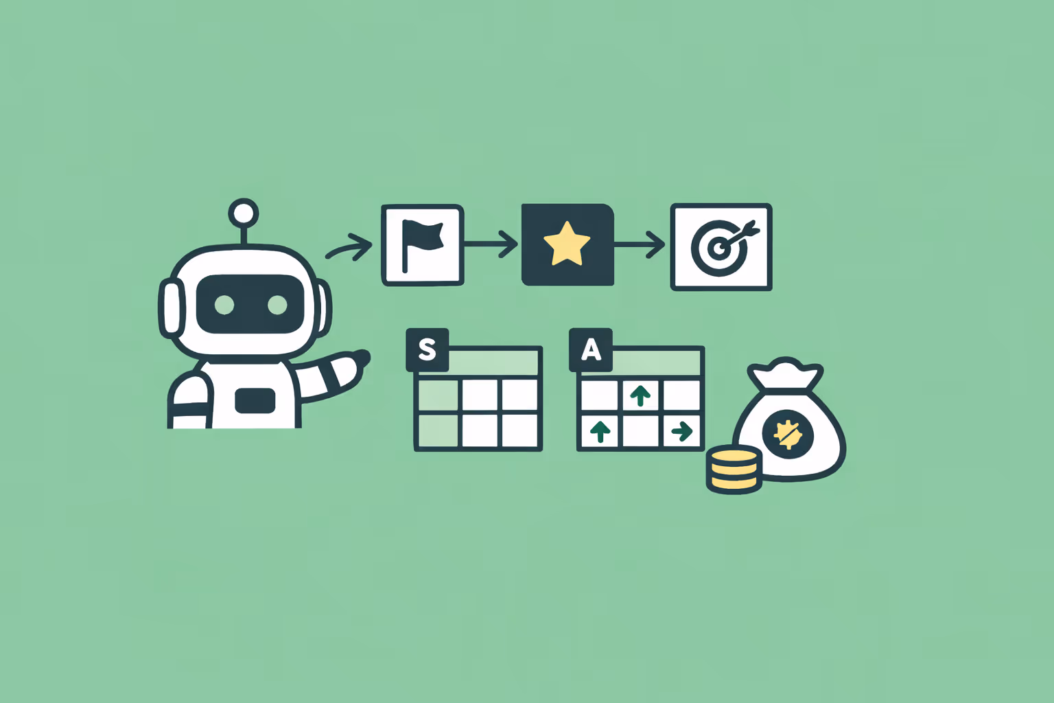
Q-learning is a model-free reinforcement learning algorithm that teaches agents to make optimal decisions. Learn how it works, where it's used, and how to implement it.
What Is Q-Learning?
Q-learning is a model-free reinforcement learning algorithm that enables an intelligent agent to learn the optimal action to take in each state of an environment. It works by estimating a value function, called the Q-function, that assigns a numerical score to every possible state-action pair.
The "Q" stands for quality, representing how useful a given action is in a given state for maximizing future cumulative reward.
Unlike supervised learning, where a model trains on labeled input-output pairs, Q-learning operates through trial and error. The agent interacts with an environment, receives rewards or penalties for its actions, and gradually updates its Q-values to reflect which actions lead to the best long-term outcomes. No prior knowledge of the environment's dynamics is required, which is why Q-learning is classified as model-free.
Q-learning was introduced by Christopher Watkins in 1989 and has since become one of the most foundational algorithms in artificial intelligence. Its convergence guarantees under certain conditions, combined with its conceptual simplicity, make it a standard starting point for anyone learning reinforcement learning.
The algorithm forms the backbone of more advanced methods, including Deep Q-Networks (DQN), which extend Q-learning to handle high-dimensional state spaces using deep learning.
How Q-Learning Works
The Q-Table and State-Action Pairs
At the core of Q-learning is a data structure called the Q-table. This table has one row for every possible state the agent can encounter and one column for every possible action the agent can take. Each cell stores the Q-value for that particular state-action combination, representing the expected cumulative reward the agent will receive if it takes that action from that state and then follows the optimal policy thereafter.
At the start of training, Q-values are typically initialized to zero or small random numbers. As the agent explores the environment, it updates these values based on the rewards it receives and the estimated value of subsequent states. Over many episodes of interaction, the Q-table converges toward the true optimal values.
The Bellman Equation
The mathematical foundation of Q-learning is the Bellman equation for optimal Q-values. The update rule adjusts the Q-value for a state-action pair based on the immediate reward received plus the discounted maximum Q-value of the next state. The formula is:
Q(s, a) = Q(s, a) + alpha [reward + gamma max Q(s', a') - Q(s, a)]
In this equation, alpha is the learning rate, which controls how much new information overrides the existing Q-value. Gamma is the discount factor, a value between 0 and 1 that determines how much the agent values future rewards relative to immediate ones. A gamma close to 1 makes the agent far-sighted, while a gamma close to 0 makes it focus on immediate gains.
The term "max Q(s', a')" represents the highest Q-value achievable from the next state across all possible actions. This forward-looking component is what allows Q-learning to optimize for long-term cumulative reward rather than just immediate payoff.
Exploration vs. Exploitation
One of the central challenges in Q-learning is balancing exploration and exploitation. Exploitation means choosing the action with the highest known Q-value. Exploration means trying actions that may not currently appear optimal, in order to discover potentially better strategies that the agent has not yet encountered.
The most common approach is the epsilon-greedy strategy. With probability epsilon, the agent selects a random action (exploration). With probability 1 minus epsilon, it selects the action with the highest Q-value (exploitation). Epsilon typically starts high, encouraging broad exploration, and decays over time as the agent builds confidence in its Q-value estimates.
Without sufficient exploration, the agent may converge to a suboptimal policy, never discovering that a different sequence of actions leads to higher total reward. Without sufficient exploitation, the agent wastes time on random actions instead of leveraging what it has already learned.
Training Episodes and Convergence
Q-learning operates in episodes. Each episode begins with the agent in a starting state and ends when it reaches a terminal state or a maximum number of steps. During each episode, the agent selects actions, observes rewards, transitions to new states, and updates its Q-table according to the Bellman equation.
Given sufficient exploration of all state-action pairs and a learning rate that decays appropriately over time, Q-learning is mathematically guaranteed to converge to the optimal Q-values. In practice, convergence speed depends on the size of the state-action space, the reward structure, and the choice of hyperparameters.
Q-Learning vs Other RL Methods
Q-Learning vs. SARSA
SARSA (State-Action-Reward-State-Action) is another temporal-difference reinforcement learning algorithm that closely resembles Q-learning. The key difference lies in how each algorithm updates its Q-values. Q-learning is off-policy, meaning it updates based on the maximum possible Q-value of the next state regardless of which action the agent actually takes. SARSA is on-policy, updating based on the action the agent actually selects in the next state.
This distinction has practical consequences. Q-learning tends to learn more aggressive, reward-maximizing policies because it always assumes the best future action. SARSA tends to learn safer policies because it accounts for the exploration that the agent is actually doing. In environments where dangerous states exist near optimal paths, SARSA may find more cautious routes while Q-learning may find the theoretically optimal but riskier path.
Q-Learning vs. Deep Q-Networks (DQN)
Standard Q-learning stores values in a table, which works well when the number of states and actions is manageable. Many real-world problems have state spaces far too large for a table. A video game screen, for example, has millions of possible pixel configurations, making a tabular approach infeasible.
Deep Q-Networks address this limitation by replacing the Q-table with a neural network that approximates Q-values. The network takes a state as input and outputs estimated Q-values for each possible action. DQN introduced techniques like experience replay and target networks to stabilize training, and it demonstrated superhuman performance on Atari games in 2015.
Frameworks like PyTorch are commonly used to build these networks.
Q-Learning vs. Policy Gradient Methods
Q-learning and policy gradient methods represent two fundamentally different approaches to reinforcement learning. Q-learning learns a value function and derives a policy from it (choose the action with the highest Q-value). Policy gradient methods learn the policy directly, parameterizing it as a probability distribution over actions and optimizing it using gradient descent.
Policy gradient methods handle continuous action spaces more naturally. Q-learning requires discretizing actions, which becomes impractical in high-dimensional continuous domains like robotic arm control. Policy gradient methods also tend to converge more smoothly, though they often require more samples and can be sensitive to hyperparameter choices.
Actor-critic methods combine both approaches, using a value function (critic) to reduce the variance of policy gradient updates (actor). This hybrid architecture underpins many modern reinforcement learning systems.
Q-Learning vs. Supervised and Unsupervised Learning
Q-learning sits in a distinct category from both supervised and unsupervised learning. In supervised learning, a model learns from labeled examples provided in advance. In unsupervised learning, a model discovers patterns in unlabeled data. In Q-learning, the agent generates its own training data through interaction with the environment, receiving only sparse reward signals rather than explicit labels.
This makes Q-learning suitable for sequential decision-making problems where the correct action at each step depends on the long-term consequences, not just the immediate outcome. It fills a niche that neither supervised nor unsupervised methods can address directly.
| Type | Description | Best For |
|---|---|---|
| Q-Learning vs. SARSA | SARSA (State-Action-Reward-State-Action) is another temporal-difference reinforcement. | The key difference lies in how each algorithm updates its Q-values |
| Q-Learning vs. Deep Q-Networks (DQN) | Standard Q-learning stores values in a table. | Many real-world problems have state spaces far too large for a table |
| Q-Learning vs. Policy Gradient Methods | Q-learning and policy gradient methods represent two fundamentally different approaches to. | — |
| Q-Learning vs. Supervised and Unsupervised Learning | Q-learning sits in a distinct category from both supervised and unsupervised learning. | — |
Q-Learning Use Cases
Game Playing and Strategy
Q-learning first gained widespread attention through game-playing applications. DeepMind's DQN agent mastered dozens of Atari 2600 games from raw pixel input, in many cases surpassing human expert performance. The agent received only the game score as reward and learned strategies entirely through trial and error.
Board games, card games, and strategy games also benefit from Q-learning and its extensions. The algorithm naturally handles the sequential decision-making structure of turn-based games, where each move affects future options. While the most famous game-playing systems like AlphaGo use more advanced methods (Monte Carlo Tree Search combined with deep reinforcement learning), Q-learning provides the conceptual foundation for understanding value-based approaches to game AI.
Robotics and Autonomous Navigation
Robot navigation is a natural application of Q-learning. A robot operating in a warehouse, hospital, or factory must decide how to move through its environment to reach a destination while avoiding obstacles. Q-learning allows the robot to learn an optimal navigation policy through repeated interaction with the environment, either in simulation or in the real world.
Self-driving car systems use reinforcement learning principles for lane-changing decisions, intersection navigation, and speed control. While production autonomous vehicle systems rely on complex multi-component architectures, Q-learning and its deep variants inform the decision-making modules that select driving actions based on sensor observations.
Resource Management and Scheduling
Q-learning applies to resource allocation problems where decisions must be made sequentially under uncertainty. Cloud computing platforms use Q-learning to allocate server resources dynamically, balancing performance against cost. Energy grids use it to schedule power distribution across sources in response to fluctuating demand.
Job scheduling, inventory management, and supply chain optimization all involve sequential decisions where current choices affect future options. Q-learning provides a principled framework for learning scheduling policies that minimize costs or maximize throughput without requiring a complete mathematical model of the system.
Recommendation Systems and Personalization
Recommendation engines can frame content selection as a reinforcement learning problem. The agent (recommendation system) observes user state (browsing history, preferences), takes actions (recommending items), and receives rewards (clicks, purchases, engagement time). Q-learning allows the system to optimize for long-term engagement rather than just immediate clicks.
This approach is particularly valuable in education, where an autonomous AI tutor can use Q-learning to select the next lesson, exercise, or assessment for a learner based on their cumulative performance.
The algorithm optimizes the learning path for long-term knowledge retention rather than short-term quiz scores, aligning with how predictive modeling anticipates learner outcomes.
Network Routing and Telecommunications
Q-learning has been applied to network routing problems, where data packets must find optimal paths through complex communication networks. Each router acts as an agent that learns which neighbor to forward packets to, minimizing latency and avoiding congestion.
The decentralized nature of Q-learning makes it well-suited for distributed network environments where no single controller has a complete view of network state. Each node maintains its own Q-table and updates it based on local observations, naturally adapting to changing network conditions without requiring a centralized optimization model.
Challenges and Limitations
The Curse of Dimensionality
Tabular Q-learning stores a Q-value for every state-action pair, which becomes impractical as the state or action space grows. An environment with 1,000 possible states and 10 possible actions requires a table with 10,000 entries, which is manageable. An environment with a million states and 100 actions requires 100 million entries, which strains memory and dramatically slows convergence.
Function approximation methods, including DQN, address this by generalizing across similar states. However, function approximation introduces its own challenges, including training instability and the possibility of divergence.
The backpropagation algorithm used to train these approximating networks must be carefully tuned to avoid catastrophic forgetting, where learning new state-action values erases previously learned ones.
Sparse and Delayed Rewards
Q-learning struggles in environments where rewards are sparse or significantly delayed. If the agent receives a reward only upon completing a long sequence of actions, it takes many episodes for that reward signal to propagate backward through the Q-table to earlier states. During this propagation period, the agent has little guidance on which early actions contribute to eventual success.
Reward shaping, where intermediate rewards are manually designed to guide the agent, can mitigate this problem but requires domain expertise and risks introducing biases that lead to unintended behavior. Hierarchical reinforcement learning, which decomposes tasks into subtasks with their own reward structures, offers another approach.
Overestimation Bias
Standard Q-learning tends to overestimate Q-values because it uses the maximum Q-value of the next state in its update rule. When Q-values contain estimation errors (as they always do during training), taking the maximum selects the action with the largest positive error, systematically inflating value estimates.
Double Q-learning addresses this by maintaining two separate Q-tables and using one to select actions while the other provides the value estimate. This decouples action selection from value estimation and significantly reduces overestimation bias. Double DQN applies the same principle to deep Q-networks.
Continuous State and Action Spaces
Q-learning was designed for discrete states and actions. Applying it to continuous domains requires discretization, which introduces a trade-off between resolution and table size. Fine discretization captures more detail but explodes the state-action space. Coarse discretization keeps the table manageable but loses important distinctions between similar states.
For continuous problems, policy gradient methods or actor-critic architectures are generally preferred. However, understanding Q-learning remains valuable because it provides the conceptual basis for the critic component in actor-critic methods and because many real-world problems can be effectively discretized.
Sample Inefficiency
Q-learning requires a large number of interactions with the environment to converge, especially in complex settings. Each experience (state, action, reward, next state) updates only one entry in the Q-table, meaning the agent must visit every state-action pair many times to build accurate estimates.
Experience replay, where past experiences are stored and replayed during training, improves sample efficiency by allowing each experience to contribute to multiple updates. Prioritized experience replay further improves this by replaying experiences from which the agent can learn the most, based on the magnitude of the temporal-difference error.
How to Implement Q-Learning
Implementing Q-learning from scratch is straightforward and serves as an excellent introduction to reinforcement learning concepts. The process follows a clear sequence that maps directly to the algorithm's theoretical framework.
- Define the environment. Specify the set of states, the set of actions available in each state, the transition dynamics (how actions change state), and the reward function. For learning purposes, grid-world environments or OpenAI Gym's Taxi-v3 and FrozenLake environments provide well-defined starting points.
- Initialize the Q-table. Create a table with dimensions (number of states) by (number of actions). Initialize all values to zero. This table will store the agent's learned estimates of optimal state-action values.
- Set hyperparameters. Choose the learning rate (alpha), discount factor (gamma), exploration rate (epsilon), and the number of training episodes. Typical starting values are alpha = 0.1, gamma = 0.99, and epsilon = 1.0 with a decay rate that reduces epsilon toward 0.01 over training.
- Run the training loop. For each episode, reset the environment to a starting state. At each step, select an action using the epsilon-greedy strategy, execute the action, observe the reward and next state, update the Q-table using the Bellman equation, and transition to the next state. Repeat until the episode terminates.
- Decay exploration over time. After each episode, reduce epsilon by a small factor. This gradually shifts the agent from exploration toward exploitation as its Q-value estimates improve. A common approach multiplies epsilon by a decay rate (such as 0.995) after each episode.
- Evaluate the learned policy. After training, set epsilon to zero so the agent always selects the action with the highest Q-value. Run the agent through several test episodes and measure its average cumulative reward. Compare this against a random policy to verify that learning has occurred.
- Scale with function approximation. Once comfortable with tabular Q-learning, replace the Q-table with a neural network to handle larger state spaces. Machine learning frameworks like PyTorch make this transition manageable by providing the necessary building blocks for defining networks, computing losses, and running gradient descent updates.
Practitioners working with Q-learning often find it helpful to visualize the Q-table during training to understand how values propagate from rewarding terminal states back to earlier states. Heatmap visualizations of Q-values across a grid world provide immediate intuition for how the algorithm learns.
FAQ
Is Q-learning the same as reinforcement learning?
Q-learning is one specific algorithm within the broader field of reinforcement learning. Reinforcement learning encompasses many approaches, including policy gradient methods, actor-critic methods, Monte Carlo methods, and temporal-difference learning. Q-learning falls under the temporal-difference category and is specifically a value-based, off-policy method.
It is one of the most widely taught RL algorithms, but it is not synonymous with reinforcement learning as a whole.
Can Q-learning handle continuous action spaces?
Standard tabular Q-learning requires discrete states and actions. Continuous action spaces must either be discretized (divided into bins) or handled using function approximation methods like Deep Q-Networks. For truly continuous action problems, such as controlling the torque of a robotic joint, policy gradient or actor-critic methods like DDPG (Deep Deterministic Policy Gradient) or SAC (Soft Actor-Critic) are generally more appropriate.
How long does Q-learning take to converge?
Convergence time depends on the size of the state-action space, the reward structure, and the hyperparameter settings. A simple grid world with a few dozen states may converge in a few hundred episodes. A complex environment with thousands of states may require millions of episodes.
Guaranteed convergence requires that every state-action pair is visited infinitely often and that the learning rate satisfies certain decay conditions, though practical implementations use approximations of these requirements.
What is the difference between Q-learning and Deep Q-Networks?
Q-learning uses a lookup table to store Q-values for every state-action pair. Deep Q-Networks (DQN) replace this table with a neural network that generalizes across states, enabling the algorithm to handle environments with very large or continuous state spaces. DQN also introduces experience replay and target networks to stabilize training.
The underlying principle, learning Q-values via the Bellman equation, remains the same in both approaches.
Is Q-learning still relevant with modern AI advances?
Q-learning remains highly relevant both as a learning tool and as a practical algorithm. It provides the conceptual foundation for understanding value-based reinforcement learning, which underpins many modern systems. Deep Q-Networks, Double DQN, Dueling DQN, and Rainbow are all direct extensions of Q-learning. For problems with manageable discrete state-action spaces, tabular Q-learning is computationally efficient and interpretable.
Its principles also inform the critic component of actor-critic architectures used in state-of-the-art systems.
Further reading

Artificial General Intelligence (AGI): What It Is and Why It Matters
Artificial general intelligence (AGI) refers to AI that matches human-level reasoning across any domain. Learn what AGI is, how it differs from narrow AI, and why it matters.
What Is Neuromorphic Computing? Definition, Architecture, and Applications
Learn what neuromorphic computing is, how brain-inspired chips process information using spiking neural networks, and why this architecture matters for energy-efficient AI at the edge.

Automated Reasoning: What It Is, How It Works, and Use Cases
Automated reasoning uses formal logic and algorithms to prove theorems, verify software, and solve complex problems. Explore how it works, types, and use cases.

AgentOps: Tools and Practices for Managing AI Agents in Production
Learn what AgentOps is, why it matters for AI agent deployments, the core components of observability, cost tracking, and governance, and how to implement AgentOps in your organization.
What Is Computational Linguistics? Definition, Careers, and Practical Guide
Learn what computational linguistics is, how it bridges language and computer science, its core techniques, real-world applications, and career paths.

What Is Unsupervised Learning? Types, Methods, and Use Cases
Unsupervised learning finds hidden patterns in unlabeled data. Learn how clustering, dimensionality reduction, and association methods work across real-world applications.