What Are Graph Neural Networks?

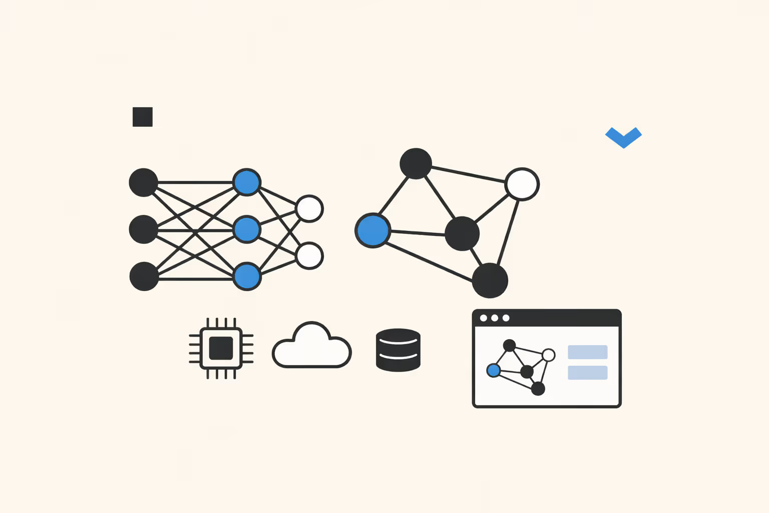
Graph neural networks are a class of deep learning models designed to operate directly on graph-structured data. A graph consists of nodes (also called vertices) and edges (the connections between them). Unlike images, which have a fixed grid structure, or text, which follows a linear sequence, graphs can represent irregular, non-Euclidean relationships where each node may connect to any number of neighbors in any configuration.

The fundamental principle behind graph neural networks is that a node's meaning depends on its context within the graph. GNNs learn representations for each node by aggregating information from neighboring nodes, a process commonly called message passing. After several rounds of message passing, each node accumulates a rich embedding that encodes both its own features and the structural patterns of its local neighborhood.

This makes graph neural networks distinct from architectures like convolutional neural networks, which assume spatial regularity, and recurrent neural networks, which assume sequential order. GNNs impose no such assumptions.

They handle data where relationships are the primary source of information: social networks, molecular structures, transportation systems, knowledge graphs, and communication networks. This flexibility has made GNNs one of the most active research areas in artificial intelligence.

How Graph Neural Networks Work

Graph Representation

Every GNN begins with a graph defined by three elements: a set of nodes, a set of edges connecting pairs of nodes, and feature vectors associated with each node (and optionally each edge). A social network graph might have users as nodes, friendships as edges, and profile attributes as node features. A molecular graph might have atoms as nodes, chemical bonds as edges, and atomic properties as node features.

The graph is typically represented computationally as an adjacency matrix (indicating which nodes are connected) paired with a feature matrix (containing the feature vector for each node). Sparse representations are used for large graphs to avoid storing the full adjacency matrix in memory.

Message Passing

Message passing is the core mechanism that distinguishes graph neural networks from other neural network architectures. At each layer of a GNN, every node collects information from its immediate neighbors, transforms that information, and updates its own representation accordingly.

The process follows three steps per layer. First, each node sends a message to its neighbors, typically a transformed version of its current feature vector. Second, each node aggregates the messages it receives, using an operation like summation, averaging, or taking the maximum. Third, each node updates its own feature vector by combining the aggregated message with its previous representation, usually through a learnable function followed by a nonlinear activation.

After one round of message passing, each node's representation reflects information from its direct neighbors. After two rounds, it captures two-hop neighborhood information. After k rounds, each node has an effective receptive field of k hops. This iterative neighborhood expansion is how GNNs learn structural patterns without requiring the entire graph to be processed at once.

Training and Optimization

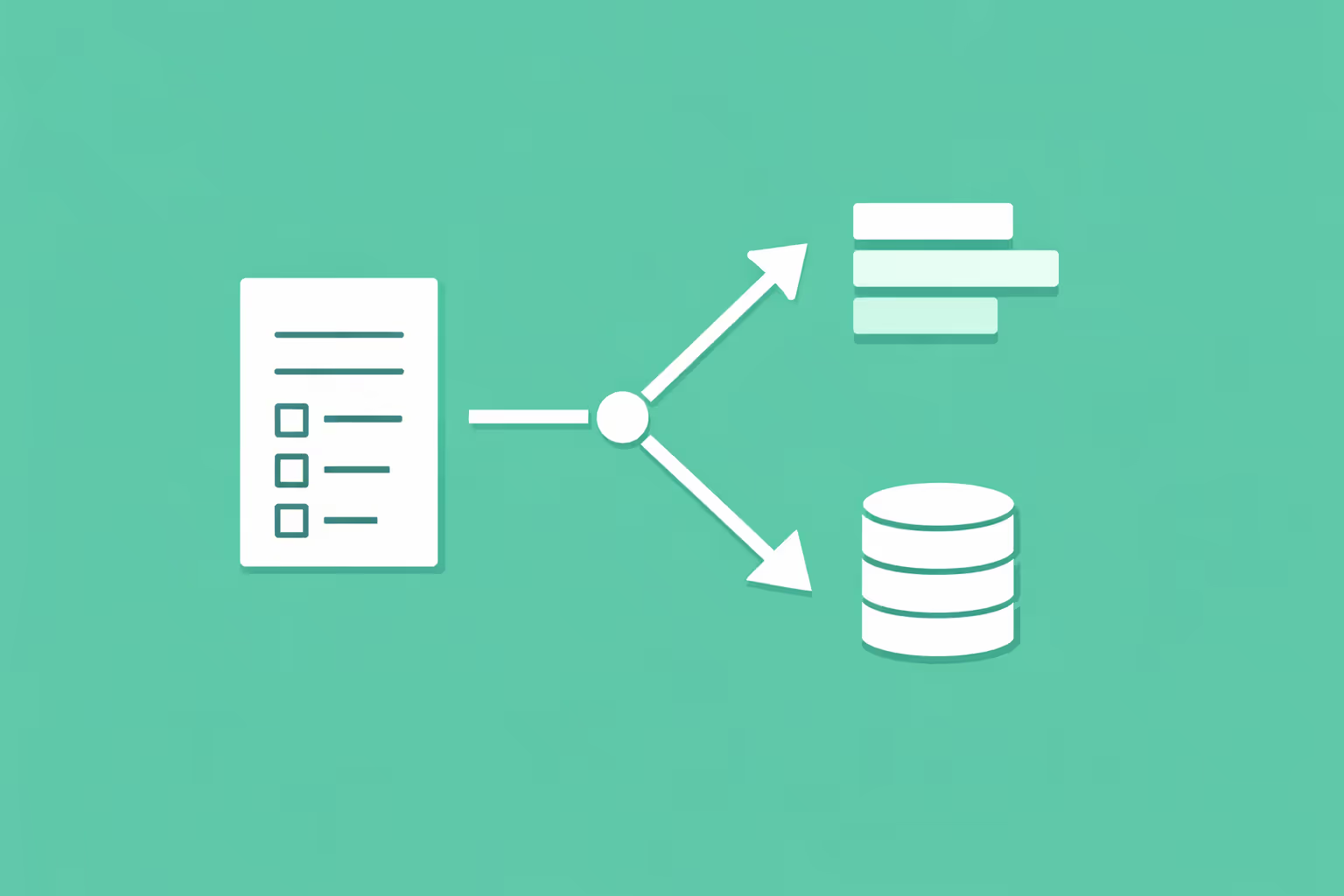
GNNs are trained using standard supervised learning or unsupervised learning techniques, depending on the task. For node classification, the loss function compares predicted node labels against ground truth. For link prediction, the model learns to score whether two nodes should be connected.

For graph classification, node embeddings are pooled into a single graph-level representation and passed through a classifier.

The learnable parameters in GNN layers are optimized through backpropagation and gradient descent, just as in other deep learning architectures. The computational graph follows the message passing structure, and gradients flow back through the aggregation and transformation functions at each layer.

Mini-batch training on large graphs requires specialized sampling strategies because nodes are interconnected. Methods like GraphSAGE's neighbor sampling and Cluster-GCN's graph partitioning allow training on subsets of the graph while preserving enough neighborhood context for meaningful message passing.

Types of Graph Neural Networks

Several GNN variants have been developed, each addressing different aspects of graph learning. The choice of architecture depends on the task, the graph's properties, and computational constraints.

Graph Convolutional Networks (GCNs)

Graph Convolutional Networks, introduced by Kipf and Welling in 2017, extend the idea of convolutions from grid-structured data to arbitrary graphs. A GCN layer computes a new node representation by averaging the features of its neighbors (including itself), applying a linear transformation, and passing the result through an activation function. GCNs are conceptually simple and computationally efficient, making them a natural starting point for graph learning tasks.

The primary limitation of GCNs is that all neighbors contribute equally to a node's updated representation. This uniform weighting means the model cannot learn to prioritize more informative neighbors over less relevant ones, which reduces expressiveness in heterogeneous graphs where neighbor importance varies.

Graph Attention Networks (GATs)

Graph Attention Networks address the equal-weighting limitation of GCNs by introducing an attention mechanism. During message passing, a GAT computes an attention coefficient for each edge, determining how much weight each neighbor's message receives. These attention weights are learned during training, allowing the model to focus on the most relevant connections for each node.

The attention mechanism in GATs is conceptually related to the self-attention used in transformer models, but operates over graph topology rather than sequence position. Multi-head attention, where multiple independent attention computations run in parallel, further increases the model's capacity to capture different types of relational patterns.

GraphSAGE

GraphSAGE (SAmple and aggreGatE) was designed for inductive learning on large graphs. Unlike GCNs and GATs, which require the full graph during training, GraphSAGE samples a fixed number of neighbors at each layer and learns an aggregation function that can generalize to unseen nodes. This makes it practical for graphs that evolve over time, such as social networks where new users appear regularly.

GraphSAGE supports multiple aggregation functions, including mean, LSTM-based, and max-pooling aggregators. Its sampling-based approach also significantly reduces memory requirements, enabling training on graphs with millions of nodes.

Message Passing Neural Networks (MPNNs)

Message Passing Neural Networks, proposed by Gilmer et al. in 2017, provide a general framework that unifies most spatial GNN approaches. MPNNs define message passing in terms of abstract message functions and update functions, where specific choices of these functions recover GCNs, GATs, and other variants as special cases.

This framework is particularly influential in computational chemistry, where molecular graphs require edge features (bond types) and global readout functions to produce graph-level predictions. MPNNs formalized the design space and made it easier to develop task-specific architectures.

Spectral Graph Neural Networks

Spectral approaches define graph convolutions in the frequency domain using the graph Laplacian's eigenvalues and eigenvectors. ChebNet approximates spectral convolutions using Chebyshev polynomials, avoiding the expensive eigendecomposition of the full Laplacian. GCNs can be interpreted as a first-order approximation of spectral graph convolutions.

Spectral methods provide strong theoretical foundations but face practical limitations. They are inherently transductive (tied to a specific graph structure), computationally expensive for large graphs, and less intuitive to design and debug than spatial methods.

Type	Description	Best For
Graph Convolutional Networks (GCNs)	Graph Convolutional Networks, introduced by Kipf and Welling in 2017.	Itself), applying a linear transformation
Graph Attention Networks (GATs)	Graph Attention Networks address the equal-weighting limitation of GCNs by introducing an.	Transformer models
GraphSAGE	GraphSAGE (SAmple and aggreGatE) was designed for inductive learning on large graphs.	Social networks where new users appear regularly
Message Passing Neural Networks (MPNNs)	Message Passing Neural Networks, proposed by Gilmer et al. in 2017.	This framework is particularly influential in computational chemistry
Spectral Graph Neural Networks	Spectral approaches define graph convolutions in the frequency domain using the graph.	—

Graph Neural Network Use Cases

Graph neural networks have found applications across domains where relational structure carries essential information. The following use cases represent areas where GNNs deliver measurable advantages over non-graph approaches.

Drug Discovery and Molecular Property Prediction

Molecules are naturally represented as graphs: atoms are nodes, chemical bonds are edges. GNNs predict molecular properties such as solubility, toxicity, and binding affinity directly from molecular structure, without requiring hand-engineered chemical descriptors. This accelerates drug screening by allowing researchers to evaluate millions of candidate molecules computationally before synthesizing them in the lab.

Frameworks like DeepMind's GNoME have demonstrated that GNNs can predict the stability of new materials with high accuracy, discovering hundreds of thousands of previously unknown stable structures. This work illustrates how graph neural networks can generate scientific insights at a scale that manual experimentation cannot match.

Social Network Analysis

Social platforms use GNNs for friend recommendation, community detection, and content ranking. Each user is a node; friendships, follows, and interactions form edges. GNNs learn user representations that capture both individual behavior patterns and social context, enabling more accurate predictions of who a user might want to connect with or what content they will engage with.

Community detection, which identifies tightly connected clusters within larger networks, benefits from GNNs' ability to capture multi-hop structural patterns. This extends beyond social media to organizational network analysis, where understanding communication patterns helps improve team dynamics and knowledge flow.

Fraud Detection and Anomaly Detection

Financial networks, where accounts, transactions, and merchants form a graph, are a natural fit for GNNs. Fraudulent behavior often manifests as unusual patterns in the graph structure: a cluster of new accounts all transacting with the same merchant, or a chain of rapid transfers designed to obscure the money trail.

GNNs capture these relational patterns that traditional tabular anomaly detection methods miss because they process each transaction independently.

GNN-based fraud detection systems have been deployed at scale by major payment processors and e-commerce platforms. Their ability to incorporate both transaction features and network topology provides a significant advantage in identifying sophisticated fraud rings.

Recommendation Systems

Recommendation engines increasingly model user-item interactions as bipartite graphs. Users and items are nodes; interactions (purchases, views, ratings) form edges. GNNs propagate information across this graph, learning representations that capture collaborative filtering signals: users who interact with similar items should have similar embeddings, and vice versa.

Pinterest's PinSage system, one of the first industrial-scale GNN deployments, processes a graph with billions of nodes and edges to generate item recommendations. The graph structure captures signals that matrix factorization approaches cannot, particularly higher-order interaction patterns.

Traffic and Transportation Networks

Road networks, flight routes, and public transit systems are inherently graph-structured. GNNs predict traffic flow, estimate travel times, and optimize routing by learning spatiotemporal patterns across the network. Google Maps uses a GNN-based system to improve estimated time of arrival predictions by modeling how congestion propagates through connected road segments.

The advantage of GNNs in this domain is their ability to capture how conditions at one location influence connected locations. A traffic jam on a highway ramp affects downstream surface streets in predictable patterns that GNNs can learn from historical data.

Knowledge Graph Completion

Knowledge graphs store factual information as entity-relation-entity triples. GNNs operate on these graphs to predict missing links, infer new relationships, and improve semantic search.

By learning vector embeddings for entities and relations, GNNs can answer queries about facts not explicitly stored in the graph.

This capability is central to building more complete and accurate knowledge bases, which in turn power question answering systems, search engines, and natural language processing applications that rely on structured world knowledge.

Challenges and Limitations

Over-Smoothing

The most widely discussed limitation of deep GNNs is over-smoothing. As message passing layers are stacked, node representations converge toward similar values because each node aggregates information from an exponentially growing neighborhood. After enough layers, all nodes in a connected component become nearly indistinguishable, losing the local structural information that makes them useful.

This limits practical GNN depth to roughly two to five layers for most tasks, far shallower than the deep architectures used in computer vision or language modeling. Techniques like residual connections, normalization layers, and DropEdge (randomly removing edges during training) help mitigate over-smoothing but do not fully resolve it.

Scalability

Real-world graphs can contain billions of nodes and edges. Storing the full adjacency matrix and performing message passing over the entire graph is infeasible at this scale. Neighbor sampling reduces the computational footprint but introduces variance in gradient estimates. Graph partitioning methods divide the graph into manageable subgraphs but lose cross-partition connections.

Distributed training across multiple machines adds communication overhead, particularly for message passing operations that require cross-machine node feature exchanges. Efficient large-scale GNN training remains an active engineering and research challenge.

Expressiveness and the WL Test

Standard message passing GNNs are bounded in expressiveness by the Weisfeiler-Leman (WL) graph isomorphism test. This means there are structurally different graphs that a standard GNN cannot distinguish because their message passing dynamics produce identical node representations. Higher-order GNNs and positional encodings can increase expressiveness beyond this bound, but at significant computational cost.

Understanding these theoretical limitations is important for practitioners. If a task requires distinguishing graph structures that fall outside the WL hierarchy, standard GNN architectures will underperform regardless of hyperparameter tuning or additional training data.

Limited Support for Heterogeneous and Dynamic Graphs

Most foundational GNN architectures assume homogeneous graphs where all nodes and edges are of the same type. Real-world graphs are often heterogeneous: a bibliographic network has author nodes, paper nodes, and venue nodes, each with different feature spaces and relationship types. Heterogeneous GNN extensions exist but add architectural complexity and are less mature than their homogeneous counterparts.

Dynamic graphs, where nodes and edges appear or disappear over time, present additional challenges. Temporal GNNs incorporate time-aware message passing, but maintaining up-to-date node representations as the graph evolves in real time remains computationally demanding.

Interpretability

Like other deep learning models, GNNs are difficult to interpret. Explaining why a GNN made a particular prediction requires identifying which subgraph structures and node features were most influential. Methods like GNNExplainer and PGExplainer provide post-hoc explanations by identifying important subgraphs, but these explanations are approximations and may not capture the full reasoning process.

In regulated industries where model decisions must be justified, limited interpretability can be a barrier to deployment regardless of predictive accuracy.

How to Get Started with GNNs

Getting started with graph neural networks requires a foundation in both graph theory and deep learning fundamentals. The following progression moves from conceptual understanding to practical implementation.

1. Build prerequisite knowledge. Ensure comfort with core machine learning concepts including loss functions, optimization, and overfitting. Understand basic graph theory: adjacency matrices, degree distributions, connected components, and graph traversal algorithms. Linear algebra is essential, as GNN operations are fundamentally matrix multiplications over graph structure.

2. Study the foundational papers. Read the original GCN paper by Kipf and Welling to understand how spectral graph convolutions simplify to spatial neighborhood aggregation. Then read the GAT and GraphSAGE papers to see how attention and sampling extend the basic framework. These three papers cover the core concepts that all subsequent GNN work builds upon.

3. Choose a framework. PyTorch Geometric (PyG) and Deep Graph Library (DGL) are the two leading GNN frameworks. Both integrate with PyTorch and provide implementations of standard GNN layers, benchmark datasets, and training utilities. PyG has a slightly larger ecosystem and more tutorials; DGL offers strong support for heterogeneous graphs and large-scale training.

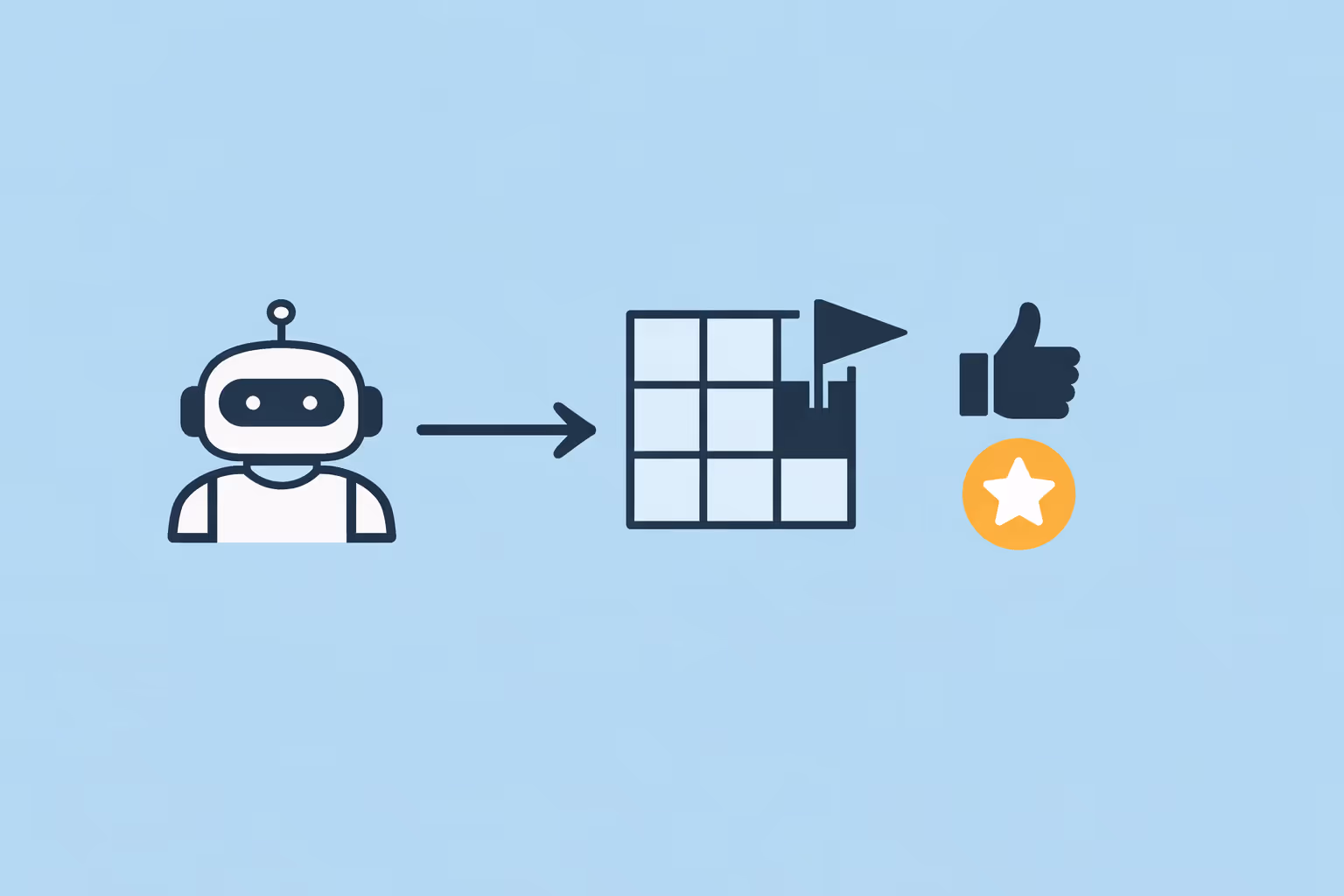
4. Implement a basic GNN from scratch. Start with node classification on a citation network like Cora or CiteSeer. Build a two-layer GCN, train it, and evaluate accuracy. Then swap in GAT layers and compare results. This hands-on exercise builds intuition for how neighborhood aggregation, layer depth, and attention affect performance.

5. Experiment with different tasks. Move beyond node classification to link prediction (predicting missing edges) and graph classification (classifying entire molecules or social network graphs). Each task type introduces different pooling strategies, loss functions, and evaluation metrics.

6. Tackle a real-world problem. Apply GNNs to a domain-specific dataset. Molecular property prediction using the OGB (Open Graph Benchmark) provides standardized leaderboards and datasets. If your interest is in recommendation systems or social networks, construct a graph from interaction data and build a GNN pipeline end to end.

7. Study scalability techniques. Once comfortable with small-graph experiments, explore mini-batch training with neighbor sampling, graph partitioning, and distributed training. These techniques are essential for any production deployment.

Teams building AI curricula can structure GNN learning paths that progress from graph fundamentals through framework proficiency to applied projects. The field is evolving rapidly, so staying current with conference proceedings from NeurIPS, ICML, and ICLR is important for practitioners who want to apply the latest techniques.

FAQ

What is the difference between a graph neural network and a regular neural network?

A regular neural network processes fixed-size inputs like vectors, images, or sequences where the structure is predefined. A graph neural network processes data organized as graphs, where the number of nodes, edges, and connections varies from instance to instance.

The key difference is the message passing mechanism: GNNs update each node's representation by aggregating information from its neighbors, allowing them to learn from relational structure that standard architectures cannot capture.

How do graph neural networks relate to transformers?

Transformer models compute attention between all pairs of tokens in a sequence, which can be viewed as operating on a fully connected graph. GNNs operate on sparse, arbitrary graph structures where connections are defined by the data rather than assumed to be universal.

Recent research has explored graph transformers that combine GNN message passing with transformer-style attention, aiming to capture both local graph structure and long-range dependencies.

What programming tools are needed for graph neural networks?

The primary tools are PyTorch Geometric (PyG) and Deep Graph Library (DGL), both built on top of PyTorch. These libraries provide efficient implementations of GNN layers, graph data structures, mini-batch loaders for large graphs, and common benchmark datasets. NetworkX is useful for graph construction and analysis, and OGB provides standardized evaluation benchmarks across multiple graph learning tasks.

Can GNNs be used for generative tasks?

Yes. Graph generative AI models can produce new graph structures, which is particularly valuable in drug discovery where generating novel molecular graphs with desired properties is the goal. Variational graph autoencoders and autoregressive graph generation models use GNN components to learn the distribution of valid graphs and sample new ones. This is an active research area with significant practical implications.

When should I use a GNN instead of a traditional machine learning model?

Use a GNN when your data has meaningful relational structure that a tabular representation would discard. If your problem involves entities with connections (users and friendships, atoms and bonds, devices and network links), and if those connections carry information relevant to the prediction task, a GNN will likely outperform models that treat each entity independently.

If your data is naturally tabular with no relational structure, standard machine learning approaches will be simpler and equally effective.