What Are Deconvolutional Networks?

Deconvolutional networks are a class of neural network architectures that reverse the spatial reduction performed by standard convolutional layers. While a convolutional neural network (CNN) progressively reduces the spatial dimensions of input data to extract high-level features, a deconvolutional network performs the inverse operation, expanding compressed feature representations back into higher-resolution spatial outputs.

The term "deconvolution" is technically a misnomer borrowed from signal processing, where it refers to reversing a convolution operation mathematically. In deep learning, the operation is more accurately called transposed convolution or fractionally strided convolution. The layer learns to upsample feature maps by inserting zeros between input values and applying learned filters, producing an output with larger spatial dimensions than the input.

A deconvolutional network typically pairs with a convolutional encoder in an encoder-decoder architecture. The encoder compresses the input into a dense feature representation. The decoder, built from transposed convolution layers, reconstructs spatial detail from that compressed representation. This pairing is the foundation of tasks that require pixel-level or spatially detailed output, from generating images to labeling every pixel in a scene.

How Deconvolutional Networks Work

The Convolution-Deconvolution Pipeline

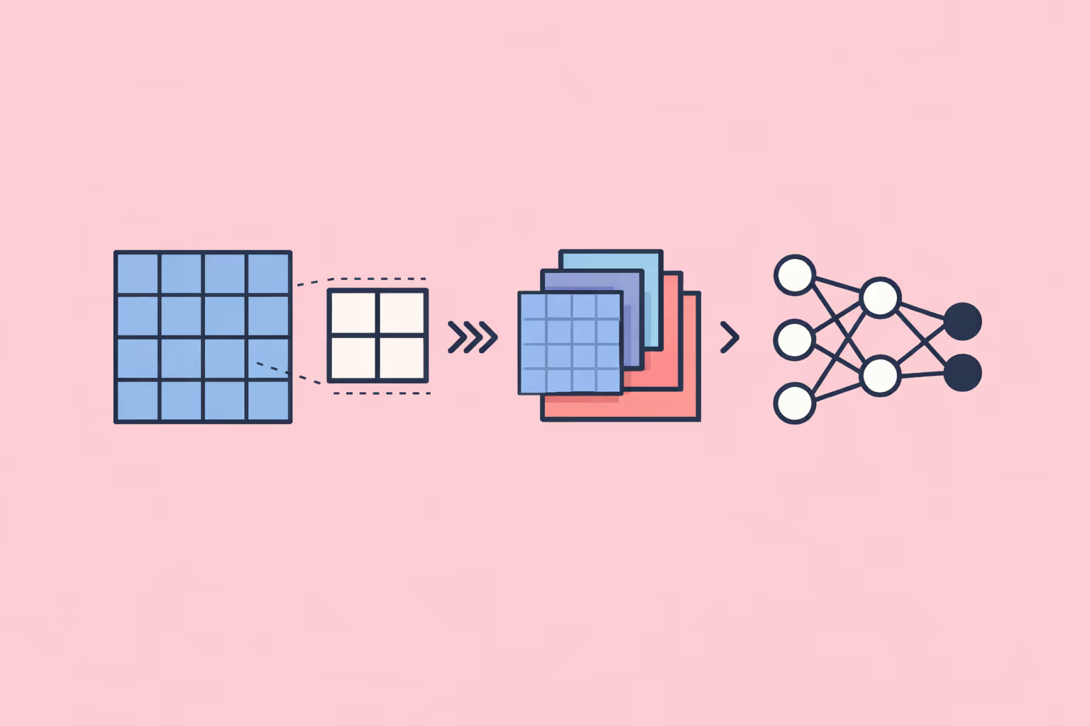
Standard convolutional layers use filters that slide across input data, producing progressively smaller feature maps. Each layer captures increasingly abstract patterns: edges become textures, textures become object parts, and object parts become semantic concepts. The spatial resolution shrinks at each stage, usually through stride operations or pooling layers.

Deconvolutional layers reverse this flow. A transposed convolution takes a small feature map and produces a larger one by learning upsampling filters. The operation effectively spreads each input value across a larger output region, with the learned filter weights determining how that spreading occurs.

Consider a 7x7 feature map at the bottleneck of a network trained on 224x224 images. The deconvolutional layers must reconstruct the full spatial resolution from that compressed 7x7 grid. Each transposed convolution layer doubles or quadruples the spatial dimensions while reducing the channel depth, progressively refining the output until it matches the target resolution.

Transposed Convolution vs. Other Upsampling Methods

Transposed convolution is not the only way to increase spatial resolution. Understanding the alternatives clarifies why transposed convolutions remain widely used despite their limitations.

- Nearest-neighbor upsampling duplicates pixel values to fill a larger grid. It is fast and parameter-free but produces blocky outputs with no learned refinement.

- Bilinear interpolation computes weighted averages of neighboring pixels for smoother upsampling. It improves on nearest-neighbor quality but still applies a fixed, non-learned transformation.

- Sub-pixel convolution (also called pixel shuffle) rearranges elements from multiple feature channels into a higher-resolution spatial grid. It avoids the checkerboard artifacts common in transposed convolutions and is popular in image super-resolution tasks.

- Transposed convolution learns its upsampling filters during training, making it adaptive to the specific task. The learned filters can recover fine details that fixed interpolation methods cannot. The trade-off is a higher parameter count and susceptibility to checkerboard artifacts when filter size and stride are not carefully matched.

In practice, many modern architectures combine these methods. A common pattern uses bilinear upsampling followed by a standard convolution, achieving learned refinement without the artifact problems of pure transposed convolution.

Skip Connections and Feature Fusion

Raw transposed convolution alone struggles to recover fine-grained spatial detail because the bottleneck representation has lost too much local information. Skip connections address this by routing feature maps from early encoder layers directly to corresponding decoder layers.

The U-Net architecture, originally developed for biomedical image segmentation, popularized this approach. Feature maps from each encoder level are concatenated with the corresponding decoder feature maps before the next transposed convolution. The decoder receives both the high-level semantic context from the bottleneck and the low-level spatial detail from the encoder, enabling precise boundary reconstruction.

Feature Pyramid Networks (FPNs) apply a similar principle at multiple scales. They merge features across different resolutions to produce predictions that are both semantically rich and spatially precise. These multi-scale fusion strategies are now standard in computer vision pipelines that require detailed spatial output.

Component	Function	Key Detail
The Convolution-Deconvolution Pipeline	Standard convolutional layers use filters that slide across input data.	—
Transposed Convolution vs. Other Upsampling Methods	Transposed convolution is not the only way to increase spatial resolution.	—
Skip Connections and Feature Fusion	Raw transposed convolution alone struggles to recover fine-grained spatial detail because.	—

Why Deconvolutional Networks Matter

Enabling Pixel-Level Predictions

Before deconvolutional architectures, convolutional networks were limited to image-level predictions: classifying an entire image as "cat" or "dog." Deconvolutional layers enabled networks to produce predictions for every individual pixel, opening up entirely new application domains.

Semantic segmentation, where each pixel receives a class label, became practical only after fully convolutional networks introduced deconvolutional layers to restore spatial resolution. Instance segmentation, depth estimation, and optical flow prediction followed, all requiring dense, pixel-wise outputs that deconvolutional architectures made feasible.

Powering Generative Models

Deconvolutional layers are central to generative models that synthesize new data. In a generative adversarial network (GAN), the generator takes a random noise vector and passes it through a series of transposed convolution layers to produce a full-resolution image. Each layer adds spatial detail, transforming abstract noise into coherent visual structure.

Variational autoencoders (VAEs) use a similar decoder structure. The latent representation sampled from the learned distribution is decoded through transposed convolutions back into image space. The quality of the generated output depends directly on how effectively the deconvolutional layers reconstruct spatial coherence from the compressed latent code.

Understanding the distinction between generative AI and predictive AI helps practitioners recognize that deconvolutional layers are not just a technical detail. They are the mechanism that gives generative networks their ability to produce spatially structured output.

Bridging Compression and Reconstruction

Every task that compresses information and later needs to reconstruct it benefits from deconvolutional architectures. Video prediction models compress temporal context and decode future frames. Medical imaging systems compress scans and reconstruct highlighted regions of interest. Autonomous driving systems compress sensor inputs and reconstruct dense scene maps for navigation decisions.

The compression-reconstruction pattern is fundamental to how deep learning handles spatial data. Deconvolutional layers are the primary mechanism for the reconstruction half of that pattern.

Use Cases and Applications

Semantic Segmentation

Semantic segmentation assigns a class label to every pixel in an image. Fully convolutional networks (FCNs) were the first architectures to demonstrate this at scale, replacing the final fully connected layers of a classification network with deconvolutional layers that restore spatial resolution.

Modern segmentation architectures like DeepLab, PSPNet, and U-Net all rely on deconvolutional or upsampling decoder stages. Applications span autonomous driving (labeling roads, vehicles, pedestrians), agriculture (crop and weed detection from aerial imagery), satellite analysis (land use classification), and medical diagnostics (tumor boundary delineation in MRI and CT scans).

The accuracy of segmentation depends on the decoder's ability to reconstruct sharp object boundaries from compressed feature maps. Skip connections and multi-scale fusion are critical for achieving the boundary precision that real-world applications demand.

Image Generation and Style Transfer

GANs and VAEs use deconvolutional decoders to generate images from latent representations. Text-to-image models, face synthesis systems, and artistic style transfer pipelines all rely on the decoder's ability to produce spatially coherent, high-resolution output from compact internal representations.

Diffusion models, which have become the dominant paradigm for high-quality image generation, also incorporate deconvolutional principles in their denoising networks. The U-Net backbone used in models like Stable Diffusion includes transposed convolution layers in its decoder path, guided by skip connections from the encoder.

Training teams working on AI-generated visual content should understand that the decoder architecture directly controls output quality, resolution, and the types of artifacts that appear in generated images.

Image Super-Resolution

Super-resolution networks reconstruct high-resolution images from low-resolution inputs. The decoder must hallucinate plausible high-frequency detail that does not exist in the input, a task that requires learned upsampling rather than simple interpolation.

Architectures like SRCNN, ESPCN, and EDSR use deconvolutional or sub-pixel convolution layers to achieve this. Applications include enhancing satellite imagery, improving medical scan resolution, restoring degraded surveillance footage, and upscaling video content for higher-resolution displays.

Object Detection and Instance Segmentation

Object detection frameworks like Mask R-CNN extend bounding box detection with a deconvolutional branch that produces a pixel-level mask for each detected object. The mask branch uses transposed convolutions to upsample region-of-interest features into a binary mask at the target resolution.

Feature Pyramid Networks pair convolutional downsampling with deconvolutional upsampling to detect objects at multiple scales. Small objects that occupy only a few pixels at the original resolution become detectable when the network combines high-resolution spatial features with high-level semantic features through the decoder pathway.

Depth Estimation and 3D Reconstruction

Monocular depth estimation networks take a single 2D image and produce a dense depth map predicting the distance of every pixel from the camera. The encoder extracts features that encode depth cues such as texture gradients, occlusion patterns, and relative object sizes. The deconvolutional decoder reconstructs the full-resolution depth map from these features.

3D reconstruction pipelines use similar encoder-decoder architectures to predict voxel occupancy, surface normals, or point cloud representations from 2D images. Autonomous vehicles, robotics, and augmented reality systems depend on these reconstructions for spatial understanding.

Challenges and Limitations

Checkerboard Artifacts

The most well-known artifact of transposed convolution is the checkerboard pattern that appears when the filter size is not evenly divisible by the stride. Overlapping output contributions from adjacent input positions create a periodic pattern of uneven magnitudes in the output.

This problem is well-documented. The standard mitigation is to use filter sizes divisible by the stride (for example, a 4x4 filter with stride 2) or to replace transposed convolution with resize-convolution, where bilinear upsampling is followed by a standard convolution. Many recent architectures avoid pure transposed convolution for this reason.

Computational Cost

Deconvolutional layers are computationally expensive. Each transposed convolution multiplies the spatial dimensions of its input while maintaining substantial channel depth, requiring significant memory and compute. For high-resolution outputs such as 4K images or dense 3D voxel grids, the computational requirements of the decoder can exceed those of the encoder.

Efficient alternatives like depthwise separable transposed convolutions, sub-pixel convolution, and progressive upsampling reduce this cost. Practitioners working within constrained environments, such as mobile deployment or edge computing, must carefully balance output quality against resource limitations.

Loss of High-Frequency Detail

Even with skip connections, deconvolutional decoders tend to produce outputs that are slightly blurred compared to ground truth. The bottleneck representation discards high-frequency spatial information that the decoder cannot fully recover. This manifests as soft edges, loss of fine texture, and smoothed details in reconstructed outputs.

Perceptual loss functions, adversarial training, and attention mechanisms help mitigate this, but the fundamental information bottleneck remains. Applications requiring pixel-perfect reconstruction, such as medical image analysis for surgical planning, must account for this limitation in their quality assessment pipelines.

Training Instability

In generative models, the deconvolutional decoder is trained jointly with other components (discriminator in GANs, encoder in VAEs). This joint training can be unstable. Mode collapse in GANs, posterior collapse in VAEs, and vanishing gradients through deep decoder stacks are common failure modes.

Techniques such as progressive growing (starting with low-resolution output and gradually increasing), spectral normalization, and careful learning rate scheduling help stabilize training. Building robust technical training programs around these stabilization techniques is essential for teams working on generative AI projects.

How to Get Started with Deconvolutional Networks

Choosing a Framework

PyTorch and TensorFlow both provide native transposed convolution layers. In PyTorch, nn.ConvTranspose2d implements the operation with configurable kernel size, stride, padding, and output padding. In TensorFlow/Keras, Conv2DTranspose provides equivalent functionality.

Start by implementing a simple autoencoder on a standard dataset like MNIST or CIFAR-10. The encoder uses standard convolutions to compress images into a latent vector. The decoder uses transposed convolutions to reconstruct images from that vector. Measuring reconstruction loss (mean squared error or binary cross-entropy) gives immediate feedback on whether the decoder is learning effectively.

Architecture Design Decisions

Several design choices significantly affect the quality of deconvolutional outputs.

- Filter size and stride alignment. Ensure the filter size is divisible by the stride to avoid checkerboard artifacts. A 4x4 filter with stride 2 or a 6x6 filter with stride 3 are safe choices.

- Skip connections. For any task requiring precise spatial output (segmentation, depth estimation), include skip connections from encoder to decoder. U-Net's concatenation strategy is a reliable default.

- Normalization. Batch normalization after each transposed convolution layer stabilizes training. For generative models, instance normalization or group normalization may produce better results.

- Activation functions. ReLU or Leaky ReLU between decoder layers is standard. The final output layer uses sigmoid (for outputs in [0,1] range) or tanh (for [-1,1] range) depending on the target data distribution.

Evaluating Output Quality

Reconstruction quality metrics depend on the task.

- Segmentation: Intersection over Union (IoU), mean IoU, and pixel accuracy measure how well predicted masks match ground truth.

- Image generation: Frechet Inception Distance (FID) and Inception Score (IS) measure the distributional quality of generated images.

- Super-resolution: Peak Signal-to-Noise Ratio (PSNR) and Structural Similarity Index (SSIM) quantify reconstruction fidelity.

- Depth estimation: Absolute relative error and root mean squared error against ground truth depth maps are standard.

Teams developing AI-powered learning platforms and technical applications should build evaluation pipelines early. Quantitative metrics guide architecture decisions more reliably than visual inspection alone.

FAQ

What is the difference between convolution and deconvolution in neural networks?

Convolution reduces the spatial dimensions of input data by applying learned filters that extract features. Deconvolution (more accurately called transposed convolution) increases spatial dimensions by learning upsampling filters that reconstruct spatial detail from compressed feature representations. Convolution compresses; deconvolution expands. Both use learned filter weights, but they operate in opposite spatial directions.

Are deconvolutional networks the same as autoencoders?

Not exactly. An autoencoder is an architecture that combines an encoder and a decoder. Deconvolutional layers are one way to build the decoder portion of an autoencoder. Autoencoders can use other upsampling methods in their decoders, such as bilinear interpolation or sub-pixel convolution. Deconvolutional layers also appear outside autoencoders, in segmentation networks, GANs, and object detection models.

Why do transposed convolutions produce checkerboard artifacts?

Checkerboard artifacts occur when the transposed convolution filter size is not evenly divisible by the stride. Overlapping output regions receive unequal contributions from different input positions, creating a periodic pattern of intensity variation. Using filter sizes divisible by the stride or replacing transposed convolutions with resize-convolution (bilinear upsampling followed by standard convolution) eliminates this problem.

What are the best alternatives to transposed convolution?

The main alternatives are bilinear upsampling followed by a standard convolution (resize-convolution), sub-pixel convolution (pixel shuffle), and nearest-neighbor upsampling with convolution. Resize-convolution avoids checkerboard artifacts and is widely used in modern AI architectures. Sub-pixel convolution is preferred for super-resolution tasks because of its computational efficiency. The best choice depends on the specific task, quality requirements, and computational constraints.

Can deconvolutional networks work with 3D data?

Yes. Transposed convolution extends naturally to three dimensions using ConvTranspose3d in PyTorch or Conv3DTranspose in TensorFlow. 3D deconvolutional networks are used for volumetric medical image segmentation (CT and MRI scans), 3D object reconstruction from 2D images, video prediction, and voxel-based scene understanding. The computational cost scales significantly with the third spatial dimension, making efficient architecture design critical for 3D applications.