What Is a Decision Tree?

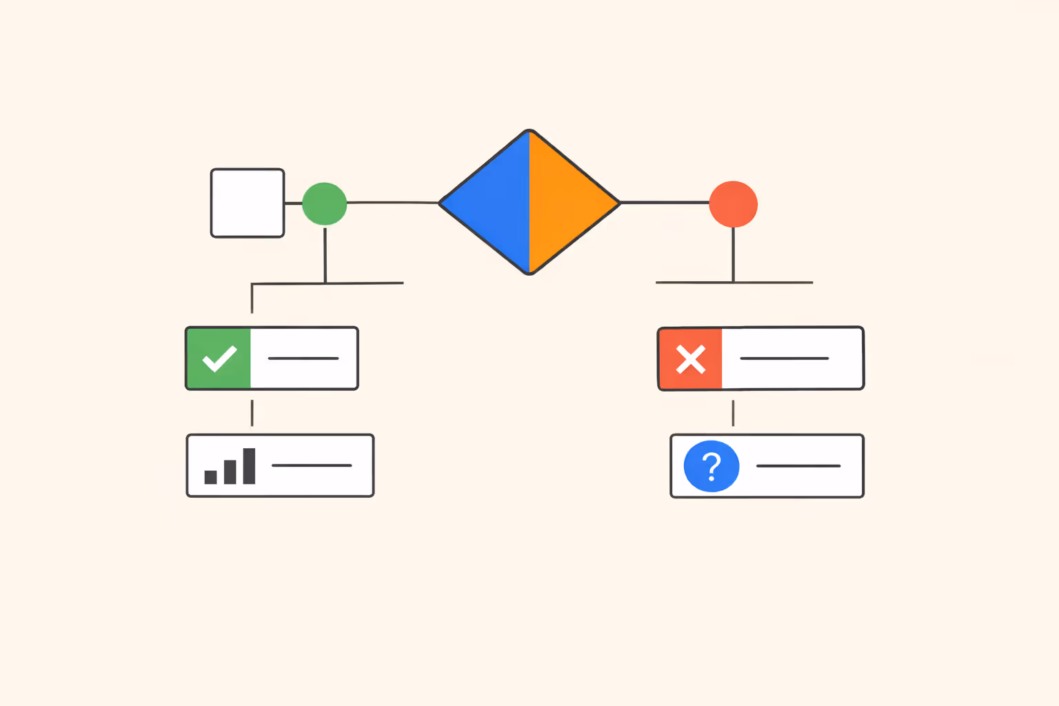
A decision tree is a supervised learning algorithm that makes predictions by splitting data through a sequence of conditional rules. Each rule tests a single feature, and the result branches into further tests until the algorithm reaches a final prediction. The output is a tree-shaped structure where every internal node represents a test on an attribute, every branch represents the outcome of that test, and every leaf node holds a predicted class label or numerical value.

The appeal of decision trees comes from their transparency. Unlike neural networks or support vector machines, a trained decision tree can be read top to bottom as a series of if-then statements. A credit risk model, for example, might first check whether the applicant's income exceeds a threshold, then check employment length, then evaluate outstanding debt. Each step is traceable, which makes the model's reasoning accessible to both technical and non-technical stakeholders.

Decision trees belong to the family of supervised learning methods, meaning they require labeled training data to learn the mapping from inputs to outputs. They handle both classification tasks (predicting a category) and regression tasks (predicting a continuous value), making them one of the most versatile structures in machine learning.

How Decision Trees Work

Building a decision tree means repeatedly partitioning the training data based on the feature that best separates the target variable at each step. The algorithm starts at the root with the full dataset, selects the most informative feature, splits the data into subsets, and recurses on each subset until a stopping condition is met.

Nodes, Branches, and Leaves

Three structural elements define every decision tree.

- Root node. The topmost node, where the first split occurs. It contains the entire training dataset and the feature test that creates the highest initial separation.

- Internal nodes. Each internal node tests a specific feature against a threshold or set of values. The test produces two or more branches, each directing a subset of the data to the next level of the tree.

- Leaf nodes. Terminal nodes where no further splitting occurs. In classification, a leaf holds the majority class of the data points that reached it. In regression, a leaf holds the mean or median of the remaining target values.

The path from root to any leaf constitutes a decision rule. A tree with five levels of depth can represent highly specific decision logic without requiring the user to write explicit conditional code.

Splitting Criteria

The quality of a decision tree depends on how it selects features and thresholds at each split. Poorly chosen splits produce shallow, uninformative separations. Well-chosen splits isolate classes or reduce variance efficiently.

For classification tasks, two metrics dominate.

- Gini impurity. Measures the probability of incorrectly classifying a randomly chosen element from the subset. A Gini impurity of zero means all elements belong to a single class. The algorithm evaluates every possible split and selects the one that minimizes the weighted Gini impurity across resulting child nodes.

- Information gain (entropy). Measures the reduction in entropy after a split. Entropy quantifies the disorder in a set of labels. Higher information gain means the split produces purer subsets. The ID3 and C4.5 algorithms use this criterion.

For regression tasks, the standard splitting criterion is variance reduction. The algorithm tests each feature and threshold combination, then selects the split that minimizes the weighted variance of the target variable across child nodes.

The choice between Gini impurity and information gain rarely produces dramatically different trees. In practice, Gini tends to favor larger partitions and is slightly faster to compute, while entropy can produce more balanced splits in multi-class problems.

Pruning and Controlling Complexity

A decision tree grown without constraints will keep splitting until every leaf contains a single training example. This produces a model that memorizes the training data but generalizes poorly to new observations. This problem is called overfitting.

Pruning addresses overfitting through two strategies.

- Pre-pruning (early stopping). Sets constraints before training begins: maximum depth, minimum samples per leaf, minimum samples required to split a node, or a minimum impurity decrease threshold. The tree stops growing when any constraint is violated. Pre-pruning is computationally efficient but requires careful tuning of hyperparameters.

- Post-pruning. Grows the full tree first, then removes branches that contribute little to predictive accuracy. Cost-complexity pruning (also called minimal cost-complexity pruning) is the most common approach. It introduces a complexity parameter that penalizes each additional leaf. Cross-validation determines the optimal complexity parameter.

Balancing tree depth against predictive power is the central trade-off. Shallow trees underfit by missing patterns. Deep trees overfit by capturing noise. Systematic tuning through cross-validation helps find the point where the model captures genuine signal without chasing artifacts.

Component	Function	Key Detail
Nodes, Branches, and Leaves	Three structural elements define every decision tree.	The topmost node, where the first split occurs
Splitting Criteria	The quality of a decision tree depends on how it selects features and thresholds at each.	For classification tasks, two metrics dominate.

- Gini impurity |

Types of Decision Trees

Decision trees split into two functional categories based on the type of target variable they predict.

Classification trees predict discrete class labels. The target variable belongs to a finite set of categories, such as "approved" or "denied," "spam" or "not spam," or diagnostic categories in medical screening. Leaf nodes in a classification tree output the majority class among the training examples that reached them. Probability estimates can also be derived from the class distribution at each leaf.

Regression trees predict continuous numerical values. Instead of class labels, the target might be a housing price, a patient's expected recovery time, or a product's demand forecast. Leaf nodes output the average (or sometimes the median) of the target values in the subset. Splitting criteria minimize variance rather than impurity.

The CART algorithm (Classification and Regression Trees), developed by Breiman, Friedman, Olshen, and Stone, handles both task types within a single framework. It uses Gini impurity for classification and variance reduction for regression, producing binary splits at every node.

Some algorithms generate multi-way splits, where a single node can branch into three or more children. C4.5, for example, creates one branch per distinct value of a categorical feature. Binary splits tend to produce deeper but more precise trees, while multi-way splits can be more interpretable when categorical features have a small number of levels.

Decision Trees in Machine Learning

Key Algorithms

Several algorithms formalize the process of building decision trees, each with distinct design choices.

- ID3 (Iterative Dichotomiser 3). Uses information gain as its splitting criterion. Handles only categorical features. Does not include a built-in pruning mechanism, which limits its robustness on noisy data.

- C4.5. An extension of ID3 that handles both categorical and continuous features. It uses gain ratio instead of raw information gain, correcting a bias toward high-cardinality features. C4.5 also includes an error-based pruning step.

- CART (Classification and Regression Trees). Produces strictly binary trees. Uses Gini impurity for classification, variance reduction for regression. Includes cost-complexity pruning. CART is the foundation for scikit-learn's DecisionTreeClassifier and DecisionTreeRegressor implementations.

- CHAID (Chi-squared Automatic Interaction Detector). Uses chi-square tests to determine splits. Designed for categorical targets and can produce multi-way splits. Often used in marketing segmentation and survey analysis.

Each algorithm reflects a set of assumptions about the data. CART's binary splits are a good default for most problems. C4.5 remains relevant when working with datasets that mix categorical and numerical features. CHAID is a specialized choice for exploratory categorical analysis.

From Single Trees to Ensemble Methods

A single decision tree is interpretable but often limited in predictive accuracy. Its greedy splitting strategy means it optimizes each split locally without considering the global structure. Small changes in the training data can produce dramatically different trees, a property known as high variance.

Ensemble methods address these limitations by combining multiple trees into a stronger collective model.

- Random forests. Train many decision trees on random subsets of both the training data (bagging) and the feature set. Each tree votes on the final prediction, and the majority vote (classification) or average (regression) determines the output. Random forests reduce variance while maintaining reasonable interpretability through feature importance scores. Understanding predictive AI systems helps contextualize how random forests fit within the broader landscape of forecasting tools.

- Gradient boosting. Trains decision trees sequentially, where each new tree corrects the errors of the previous ensemble. XGBoost, LightGBM, and CatBoost are optimized implementations that dominate tabular data competitions and production systems. Gradient boosted trees tend to achieve higher accuracy than random forests but require more careful hyperparameter tuning.

- AdaBoost. Assigns higher weights to misclassified training examples, forcing subsequent trees to focus on difficult cases. It was one of the earliest successful ensemble methods and remains useful for binary classification tasks with moderate data sizes.

The progression from a single tree to an ensemble illustrates a recurring pattern in machine learning: combining weak learners into a strong learner. A single decision tree with limited depth is a weak learner. Hundreds of such trees, combined strategically, produce models that compete with deep neural networks on structured, tabular data.

Practical Applications and Examples

Decision trees and tree-based ensembles appear across virtually every industry that works with structured data.

Credit scoring and loan approval. Banks use tree-based models to evaluate creditworthiness. Input features include income, debt-to-income ratio, employment history, and credit utilization. A decision tree can output not only the approval decision but also a traceable explanation, which is critical for compliance requirements in financial regulation.

Medical diagnosis and triage. Clinical decision support systems use decision trees to guide diagnostic workflows. A triage tree might first check patient age, then oxygen saturation, then the presence of specific symptoms. Interpretability matters here because clinicians need to verify and trust the model's logic before acting on its recommendations.

Customer churn prediction. Marketing and retention teams use gradient boosted trees to predict which customers are likely to cancel a subscription. Features typically include usage frequency, support ticket history, billing changes, and engagement metrics. The model identifies high-risk segments, enabling targeted intervention.

Manufacturing quality control. Sensor data from production lines feeds into tree-based classifiers that detect defective products. Features include temperature readings, pressure values, vibration frequencies, and timing intervals. A classification tree flags units that fall outside acceptable quality thresholds.

Fraud detection in e-commerce. Transaction data, including purchase amount, location, device type, and time of day, passes through ensemble tree models to flag suspicious activity. The speed of tree-based inference makes real-time scoring feasible even at high transaction volumes.

Teams building these systems often benefit from data science training programs that cover both the algorithmic foundations and the deployment considerations.

Education and assessment. Decision trees can model learner pathways, predicting which students are at risk of dropping out based on engagement metrics, assignment completion rates, and forum participation. Institutions that invest in adaptive testing often pair tree-based models with item response theory to personalize assessments.

Strengths and Limitations

Decision trees offer a distinct set of advantages that explain their continued popularity, alongside well-understood weaknesses that shape how practitioners use them.

Strengths

- Interpretability. A single decision tree can be visualized and explained without specialized tools. This matters in regulated industries, stakeholder communication, and training needs assessments where decisions must be justified.

- Minimal data preparation. Decision trees handle both numerical and categorical features natively. They are not sensitive to feature scaling, do not require normalization, and can tolerate missing values with appropriate imputation strategies.

- Non-linear relationships. Unlike linear models, decision trees capture interactions and thresholds automatically. A tree can represent the rule "if income is above 50K and employment length exceeds 3 years" without explicit feature engineering.

- Feature importance. Tree-based models produce natural feature importance rankings, showing which variables contribute most to predictions. This aids feature selection and domain understanding.

Limitations

- Overfitting. A single unpruned tree will memorize training data. Pruning helps, but ensembles are the more robust solution for production-grade accuracy.

- Instability. Small perturbations in training data can produce a completely different tree structure. Two datasets that differ by a handful of examples might generate trees with different root splits. Ensemble methods mitigate this, but a single tree remains inherently unstable.

- Greedy optimization. Decision trees build splits one at a time, choosing the locally optimal split without considering downstream effects. A globally suboptimal first split can cascade into a weaker overall tree. Algorithms that optimize globally, such as optimal decision trees, exist but are computationally expensive.

- Bias toward high-cardinality features. Features with many unique values can dominate splitting decisions because they offer more potential thresholds. Gain ratio (used by C4.5) and feature subsampling (used by random forests) address this bias.

- Axis-aligned boundaries. Standard decision trees split along one feature at a time, producing rectangular decision boundaries. Diagonal or curved boundaries require many splits to approximate, increasing tree depth and reducing generalization. Oblique decision trees allow splits on linear combinations of features but sacrifice some interpretability.

Understanding these trade-offs helps practitioners decide when a single tree suffices and when ensembles or alternative algorithms are necessary. For many structured data problems, gradient boosted trees represent the best balance of accuracy, speed, and explainability. For problems where full transparency is mandatory, a pruned single tree with constrained depth remains the clearest option.

Professionals developing AI-powered learning systems or building analytics into educational platforms frequently rely on tree-based models because they provide the interpretability required for stakeholder trust alongside strong baseline accuracy.

FAQ

What is the difference between a classification tree and a regression tree?

A classification tree predicts a categorical target variable, such as whether a transaction is fraudulent. It assigns each leaf node the majority class among its training examples. A regression tree predicts a continuous numerical value, such as a price or a duration. It assigns each leaf the mean of the target values in its subset. The CART algorithm handles both types, switching between Gini impurity for classification and variance reduction for regression.

When should I use a single decision tree instead of an ensemble?

Use a single decision tree when interpretability is the primary requirement and the dataset is relatively small and clean. Regulatory contexts, clinical decision support, and stakeholder-facing reports often demand fully traceable reasoning. For higher accuracy on complex or large datasets, random forests or gradient boosting methods provide better generalization at the cost of reduced transparency.

How do decision trees handle missing values?

The handling depends on the implementation. CART uses surrogate splits: when a primary feature value is missing, the algorithm substitutes a secondary feature that produces a similar partition. XGBoost and LightGBM assign missing values to whichever branch reduces loss. Some implementations require manual imputation before training. The key is to choose an algorithm whose missing-value strategy aligns with the patterns in the data.

Are decision trees suitable for high-dimensional data?

Decision trees can technically handle high-dimensional data, but performance degrades when the number of features is very large relative to the number of training examples. The search over all features and thresholds at each split becomes computationally expensive, and the risk of finding spurious splits increases. Feature selection or dimensionality reduction before training improves both speed and accuracy. Random forests partially address this by subsampling features at each split.

How deep should a decision tree be?

There is no universal answer. Depth depends on the complexity of the underlying data patterns, the number of training examples, and the tolerance for overfitting. A common approach is to train trees at multiple depths and evaluate each with cross-validation. Constraints like minimum samples per leaf or maximum number of leaf nodes offer additional control. In ensemble methods, individual trees are often limited to moderate depth (3 to 8 levels), relying on the collective to achieve accuracy.