What Is a Convolutional Neural Network?

A convolutional neural network is a class of deep learning architecture specifically designed to process data with a grid-like topology, most commonly images. Unlike standard feedforward neural networks that treat every input pixel independently, CNNs use small learnable filters that slide across the input to detect spatial patterns such as edges, textures, and shapes.

The core idea is borrowed from how the visual cortex processes information. Individual neurons in the visual cortex respond to stimuli within a restricted region of the visual field. CNNs replicate this principle computationally: each filter examines a small local patch of the input, and by stacking many such filters across multiple layers, the network builds progressively more abstract representations.

Early layers might detect horizontal edges; deeper layers recognize complex structures like faces or objects.

CNNs fall within the broader family of deep learning models and represent one of the most impactful developments in artificial intelligence. Their ability to automatically learn hierarchical features from raw pixel data, without manual feature engineering, is what made them the dominant architecture for visual recognition tasks.

How a CNN Works

Convolutional Layers

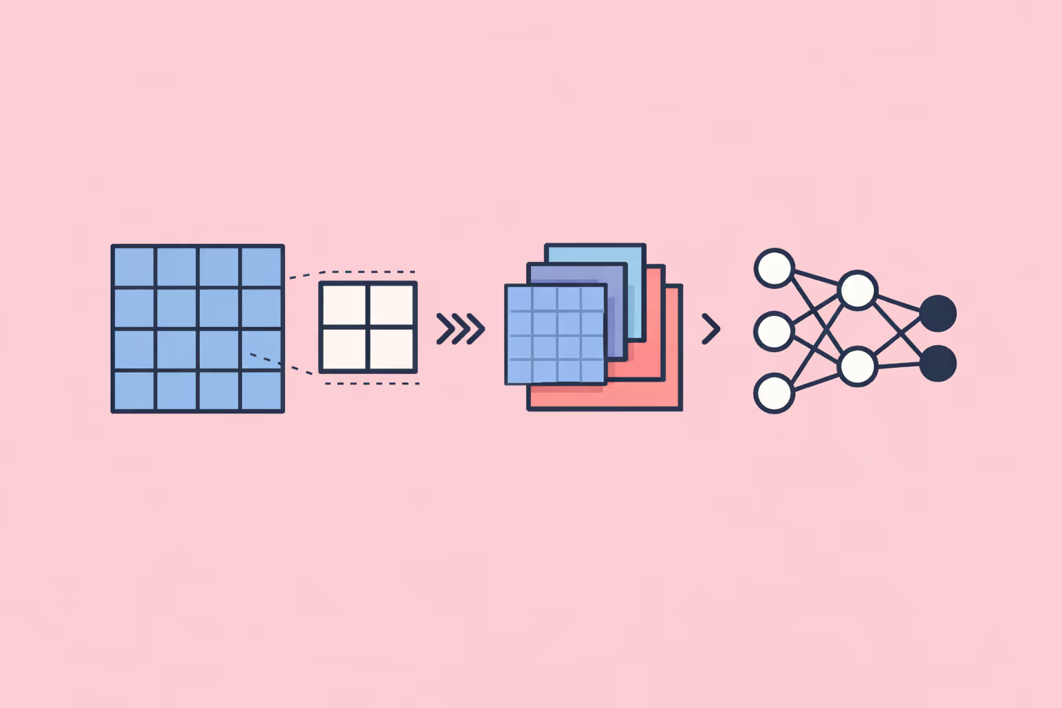
The convolutional layer is the foundational building block. It applies a set of learnable filters (also called kernels) to the input. Each filter is a small matrix, typically 3x3 or 5x5 pixels, that slides across the input image performing element-wise multiplication and summation at each position. The result is a feature map that highlights where a specific pattern occurs in the input.

A single convolutional layer usually contains dozens or hundreds of filters, each learning to detect a different feature. One filter might activate strongly on vertical edges, another on color gradients, another on corner shapes. The network learns these filters during training through backpropagation, not through manual specification.

Two important parameters control how convolutions operate. Stride determines how far the filter moves between positions. A stride of one means the filter shifts one pixel at a time; a stride of two skips every other position, producing a smaller output. Padding adds extra pixels around the input border so that the filter can process edge regions without shrinking the output dimensions.

Pooling Layers

Pooling layers reduce the spatial dimensions of feature maps while preserving the most salient information. The most common variant, max pooling, takes a small window (typically 2x2) and retains only the maximum value within that window. This operation has two practical benefits.

First, it reduces computational cost. Halving the height and width of a feature map reduces the number of values by 75%, which cascades through subsequent layers and dramatically lowers memory and processing requirements.

Second, pooling introduces a degree of translation invariance. If an edge appears slightly shifted in one image compared to another, max pooling can still produce similar feature map values because it captures the strongest activation regardless of exact position. This makes the network more robust to small variations in where objects appear within the frame.

Activation Functions

After each convolution operation, the output passes through a nonlinear activation function. Without nonlinearity, stacking multiple convolutional layers would simply produce another linear transformation, no matter how deep the network. The activation function is what allows CNNs to learn complex, nonlinear relationships in the data.

The Rectified Linear Unit (ReLU) has become the standard activation function in modern CNN architectures. ReLU sets all negative values to zero and passes positive values unchanged. Its simplicity makes computation fast, and it avoids the vanishing gradient problem that plagued earlier activation functions like sigmoid and tanh in deep networks.

Variants such as Leaky ReLU and Parametric ReLU address one of standard ReLU's weaknesses: the "dying neuron" problem, where neurons that consistently output negative pre-activation values get permanently stuck at zero. Leaky ReLU allows a small, non-zero gradient for negative inputs, keeping those neurons active during training.

Fully Connected Layers and Classification

After several rounds of convolution and pooling, the spatial feature maps are flattened into a one-dimensional vector and fed into one or more fully connected (dense) layers. These layers function identically to a traditional neural network: every neuron connects to every neuron in the previous layer.

The fully connected layers serve as the decision-making component. They take the abstract spatial features extracted by the convolutional layers and learn to map them to output categories. For an image classification task, the final fully connected layer has as many neurons as there are classes, and a softmax function converts raw scores into probability distributions across those classes.

This two-phase architecture, convolutional feature extraction followed by dense classification, is what gives CNNs their effectiveness. The convolutional layers do the perceptual heavy lifting, while the fully connected layers handle the reasoning.

Component	Function	Key Detail
Convolutional Layers	The convolutional layer is the foundational building block.	Each filter is a small matrix, typically 3x3 or 5x5 pixels
Pooling Layers	Pooling layers reduce the spatial dimensions of feature maps while preserving the most.	The most common variant, max pooling
Activation Functions	After each convolution operation.	Leaky ReLU and Parametric ReLU address one of standard ReLU's
Fully Connected Layers and Classification	After several rounds of convolution and pooling.	—

Why CNNs Matter

CNNs solved a problem that traditional machine learning approaches could not: learning visual representations directly from raw data at scale. Before CNNs, image recognition required domain experts to manually engineer features, a slow, fragile, and task-specific process.

The practical impact spans multiple dimensions.

Accuracy on visual tasks improved dramatically. On the ImageNet benchmark, a standard test of image classification across 1,000 categories, CNN-based architectures reduced error rates from roughly 25% to below 3%, surpassing average human performance. This was not a marginal improvement; it was a categorical shift in what automated systems could do with visual data.

Processing speed scaled with hardware. CNNs perform highly parallelizable matrix operations that map well onto GPUs. As GPU hardware improved, training times dropped from weeks to hours, making large-scale visual recognition practical for production systems.

Transfer learning made CNNs accessible beyond research labs. A model trained on millions of images can be fine-tuned for a new task with relatively few domain-specific examples. This means organizations do not need massive labeled datasets to build effective visual recognition systems. They can start with a pretrained backbone and adapt it, reducing both data requirements and training costs.

For teams building AI-powered learning programs, understanding CNNs is increasingly important as visual AI becomes embedded in educational tools, from automated grading of handwritten assignments to adaptive content delivery based on learner interaction patterns.

CNN Architectures That Shaped the Field

Several landmark architectures illustrate how CNN design has evolved.

LeNet-5 was one of the earliest practical CNNs, developed for handwritten digit recognition. It used a simple sequence of convolutions, pooling, and fully connected layers. LeNet proved that learned filters could outperform hand-crafted features for digit classification, but it was limited to small grayscale images.

AlexNet demonstrated that CNNs could scale. Using ReLU activation, dropout regularization, and GPU training, AlexNet won the ImageNet competition with a significant margin over non-CNN methods. It established the blueprint that deeper networks with more parameters, trained on large datasets with powerful hardware, could achieve substantially better results.

VGGNet pushed depth further with 16 to 19 layers, all using small 3x3 filters. VGG showed that stacking many small filters creates the same receptive field as fewer large filters, but with more nonlinearities and fewer parameters. The trade-off was computational cost: VGG models are large and slow compared to later architectures.

ResNet (Residual Networks) solved the degradation problem that occurs when networks get very deep. By introducing skip connections, which add the input of a layer directly to its output, ResNet allowed gradients to flow through the network without degradation. This enabled training of networks with over 100 layers, reaching new accuracy benchmarks.

EfficientNet took a different approach by systematically scaling depth, width, and resolution together using a compound scaling method. Rather than simply making networks deeper, EfficientNet optimized all three dimensions simultaneously, achieving better accuracy with fewer parameters and less computation than previous architectures.

Each of these architectures contributed a principle that modern practitioners still apply. Depth matters, but only with proper gradient flow. Small filters are generally preferable. Scaling should be balanced across dimensions. These are not abstract lessons; they are practical decisions that affect training time, inference speed, and deployment feasibility.

Real-World Applications

Medical Imaging

CNNs analyze medical scans, from chest X-rays and mammograms to retinal fundus images and pathology slides. In radiology, CNN-based systems assist clinicians by flagging potential abnormalities for review. Research has shown that certain CNN models can detect diabetic retinopathy in retinal images with sensitivity comparable to expert ophthalmologists.

The critical point for medical applications is that CNNs function as decision support, not autonomous diagnosticians. They prioritize cases, reduce review time, and catch findings that might be missed in high-volume workflows. Deployment requires rigorous validation, regulatory approval, and integration into clinical workflows.

Autonomous Vehicles

Self-driving systems use CNNs to process camera feeds in real time. Object detection networks identify pedestrians, vehicles, lane markings, and traffic signs from continuous video streams. Architectures like YOLO (You Only Look Once) and SSD (Single Shot Detector) are designed for the speed constraints of real-time driving, processing frames in milliseconds.

The challenge in this domain is not just accuracy but reliability under varying conditions: rain, fog, night driving, unusual road configurations. CNNs must generalize across conditions they may not have encountered during training, which remains an active area of applied research.

Natural Language Processing

Although transformers now dominate language tasks, CNNs still play a role in text processing. One-dimensional convolutions applied to sequences of word embeddings can capture local n-gram patterns effectively. CNNs remain competitive for text classification tasks where capturing local phrase patterns matters more than long-range dependencies.

In practice, modern NLP pipelines sometimes combine convolutional and transformer components, using CNNs for initial feature extraction and transformers for contextual reasoning.

Manufacturing and Quality Control

CNNs power visual inspection systems on production lines. They identify surface defects, dimensional deviations, and assembly errors by analyzing images of products at high speed. Compared to rule-based machine vision systems, CNN-based inspectors adapt more easily to new product types and can detect subtle defects that fixed rules miss.

Organizations building training programs for manufacturing teams increasingly include CNN-based visual inspection as a core competency area, as these systems become standard in modern factories.

Challenges and Limitations

Data Requirements

CNNs are data-hungry. Training a high-performing image classifier from scratch typically requires tens of thousands to millions of labeled examples. Collecting and annotating visual data is expensive and time-consuming, particularly in specialized domains like medical imaging or industrial inspection where expert annotators are needed.

Transfer learning mitigates this somewhat, but it does not eliminate the need for domain-specific labeled data entirely. Fine-tuning a pretrained model still requires hundreds to thousands of domain-relevant examples to achieve reliable performance.

Computational Cost

Training large CNN architectures requires significant GPU resources. ResNet-152 has over 60 million parameters; EfficientNet-B7 has 66 million. Training these models on large datasets can consume thousands of GPU-hours, with proportional energy costs.

Inference is generally faster than training, but real-time applications impose strict latency constraints. Deploying CNNs on edge devices, such as mobile phones or embedded systems, requires model compression techniques like pruning, quantization, and knowledge distillation.

Interpretability

CNNs are often described as black boxes. While techniques like Grad-CAM and saliency maps can visualize which image regions most influenced a prediction, these explanations are approximate. They show correlation, not causation.

In high-stakes domains like healthcare and criminal justice, limited interpretability is a serious concern. Practitioners must consider whether a CNN's accuracy justifies deployment in contexts where understanding the reasoning behind decisions is legally or ethically required. This connects to broader questions about AI governance and responsible deployment.

Adversarial Vulnerability

CNNs are susceptible to adversarial examples: carefully crafted input perturbations, often imperceptible to humans, that cause the model to make confident but incorrect predictions. A stop sign with a few strategically placed stickers might be classified as a speed limit sign. Understanding adversarial machine learning is essential for any team deploying CNNs in security-sensitive applications.

Defending against adversarial attacks remains an open research problem. Adversarial training, where the model is trained on both clean and adversarial examples, improves robustness but increases training cost and does not guarantee immunity.

How to Get Started with CNNs

Getting started with CNNs involves a progression from foundational concepts to hands-on implementation.

1. Build prerequisite knowledge. Understand linear algebra (matrix operations, dot products), calculus (partial derivatives for backpropagation), and probability. These are not optional. Without them, CNN behavior remains opaque.

2. Learn a deep learning framework. PyTorch and TensorFlow are the two dominant options. PyTorch is favored in research for its dynamic computation graph and Pythonic interface. TensorFlow, particularly through Keras, provides a higher-level API that simplifies prototyping.

3. Start with a standard dataset. MNIST (handwritten digits), CIFAR-10 (small color images in 10 classes), or Fashion-MNIST provide structured starting points. Build a simple CNN from scratch: two convolutional layers, max pooling, and a fully connected classifier. Train it, evaluate it, and examine where it fails.

4. Experiment with pretrained models. Load a pretrained ResNet or EfficientNet and fine-tune it on a custom dataset. This exercise demonstrates transfer learning in practice and reveals how much less data you need when starting from a pretrained backbone.

5. Study failure modes. Deliberately test your model on edge cases: rotated images, occluded objects, out-of-distribution inputs. Understanding where and why CNNs fail is as important as understanding where they succeed.

6. Explore deployment. Convert a trained model to ONNX or TensorFlow Lite format and run inference on a mobile device or edge board. The gap between a working Jupyter notebook and a production-ready system is substantial, and navigating that gap is a critical skill.

Teams structuring learning paths around AI can use resources like data science bootcamps or build custom curricula that progress from image classification basics to production deployment.

FAQ

What is the difference between a CNN and a regular neural network?

A standard feedforward neural network treats each input feature independently and connects every neuron to every neuron in adjacent layers. A CNN introduces convolutional layers that preserve spatial relationships and use shared-weight filters to detect local patterns. This weight sharing drastically reduces the number of parameters compared to fully connected alternatives and makes CNNs far more effective for structured data like images, where spatial locality matters.

Can CNNs be used for tasks other than image recognition?

Yes. CNNs process any data with spatial or sequential structure. Audio spectrograms, time series data, and text sequences can all be processed with one-dimensional or two-dimensional convolutions. In natural language processing, CNNs capture local phrase patterns in text. In genomics, one-dimensional CNNs identify patterns in DNA sequences. The core operation, sliding a filter across structured input, generalizes beyond images.

How much data is needed to train a CNN?

Training from scratch on a complex task typically requires tens of thousands to millions of labeled examples. With transfer learning, fine-tuning a pretrained model for a specific domain can produce strong results with as few as a few hundred to a few thousand labeled examples, depending on how similar the new task is to the original training domain. Data augmentation techniques like rotation, cropping, and color jittering can further stretch limited datasets.

Are CNNs still relevant given the rise of transformers?

CNNs remain highly relevant, particularly in applications where computational efficiency and real-time processing matter. Vision transformers (ViTs) have shown competitive or superior results on large-scale benchmarks, but they typically require more data and compute. Many production systems use hybrid approaches that combine convolutional feature extraction with transformer-based attention.

CNNs also maintain advantages in edge deployment scenarios where model size and inference speed are constrained.

What skills are needed to work with CNNs professionally?

Working with CNNs requires proficiency in Python, comfort with a deep learning framework (PyTorch or TensorFlow), understanding of linear algebra and calculus, and familiarity with training procedures including learning rate scheduling, regularization, and data augmentation. For deployment, knowledge of model optimization techniques, containerization, and inference serving frameworks adds practical value.

Teams can develop these competencies through structured professional development programs that combine theory with hands-on projects.