What Is Clustering in Machine Learning?

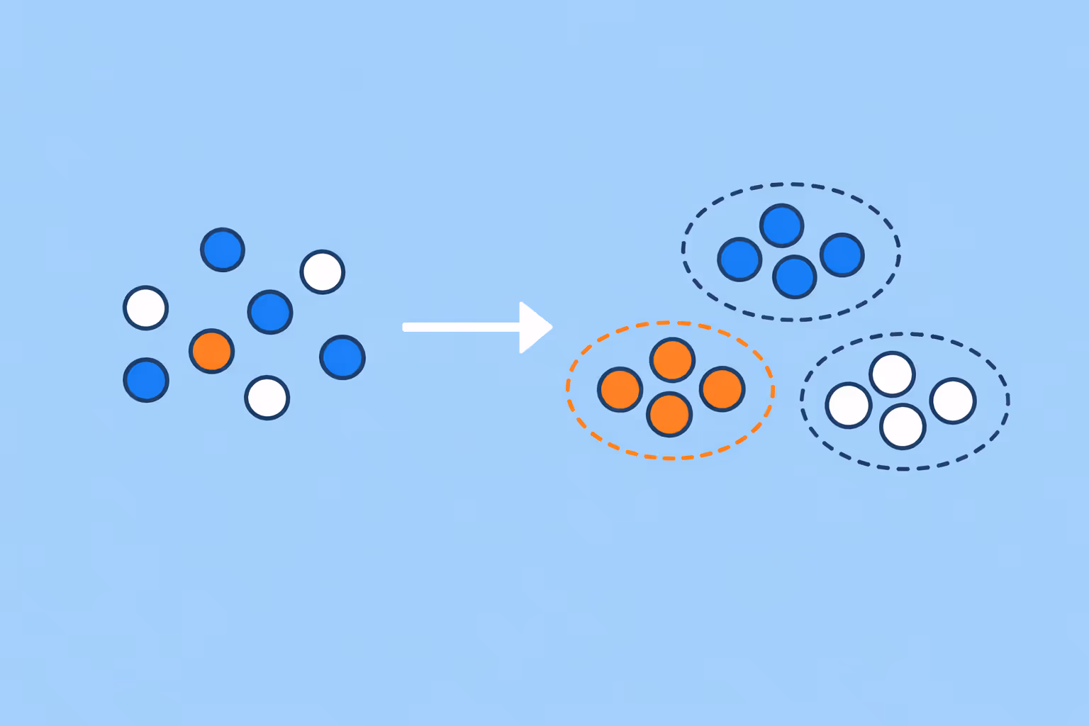
Clustering is an unsupervised learning technique that groups data points based on their similarity, without relying on predefined labels. The goal is to partition a dataset so that items within the same group (called a cluster) share more in common with each other than with items in other groups.

Unlike supervised methods such as classification or regression, clustering operates without a target variable. There is no ground truth telling the algorithm which group a data point belongs to. Instead, the algorithm discovers structure by measuring distances, densities, or statistical distributions across the feature space.

This distinction matters. Supervised learning answers "what label does this example have?" Clustering answers "what natural groupings exist in this data?" The practical consequence is that clustering is most valuable when the structure of a dataset is unknown, when labels are expensive to obtain, or when the objective is exploration rather than prediction.

Clustering appears across nearly every domain that generates structured data, from customer segmentation in marketing to gene expression analysis in biology. Understanding different types of AI helps clarify where clustering sits within the broader landscape: it belongs to the category of techniques that extract patterns from data without human-labeled examples.

How Clustering Algorithms Work

All clustering algorithms share a common goal, but they reach it through different mechanisms. The differences come down to how each method defines what "similar" means and how it assigns data points to groups.

Distance-based approaches define similarity as proximity in a feature space. Two data points are considered similar if the distance between them (Euclidean, Manhattan, or cosine distance) is small. K-Means is the most familiar example. It assigns each point to the nearest centroid, then iteratively updates centroids until assignments stabilize.

Density-based approaches define clusters as regions of high density separated by regions of low density. Rather than measuring distance to a center, they identify areas where data points are packed closely together. DBSCAN is the standard method in this family.

Distribution-based approaches assume data is generated from a mixture of probability distributions. Each cluster corresponds to one distribution, and the algorithm estimates the parameters that best explain the observed data. Gaussian Mixture Models fall into this category.

Hierarchical approaches build a nested sequence of clusters, either by starting with every point in its own cluster and merging (agglomerative) or by starting with one cluster and splitting (divisive). The result is a tree-like structure called a dendrogram that reveals relationships at multiple levels of granularity.

Each family makes different assumptions about the shape, size, and density of clusters. No single approach works best in all situations. The choice depends on the data's structure, dimensionality, and the specific problem being solved.

Major Clustering Methods

K-Means Clustering

K-Means is the most widely used clustering algorithm, largely because it is fast, intuitive, and easy to implement. It works by partitioning data into a predefined number (K) of clusters. The algorithm initializes K centroids, assigns each data point to the nearest centroid, recalculates centroids as the mean of assigned points, and repeats until convergence.

The algorithm's strength is computational efficiency. It scales linearly with the number of data points, making it practical for large datasets. Its weakness is that it assumes clusters are roughly spherical and equally sized. Elongated, overlapping, or irregularly shaped clusters will be poorly represented.

K-Means also requires the user to specify K in advance. Choosing the wrong value produces misleading results. The elbow method and silhouette analysis are two common techniques for estimating the optimal number of clusters, but neither is foolproof.

K-Medoids is a related variant that uses actual data points as cluster centers rather than computed means. This makes K-Medoids more robust to outliers because extreme values do not pull the center away from the cluster's true location.

Hierarchical Clustering

Hierarchical clustering builds a tree of nested cluster assignments, giving analysts a view of how data groups at different levels of similarity. Agglomerative (bottom-up) hierarchical clustering starts with each data point as its own cluster and progressively merges the two closest clusters until one remains.

The choice of linkage criterion determines how "closeness" between clusters is measured:

- Single linkage uses the minimum distance between any two points in different clusters. It can handle elongated shapes but is sensitive to noise.

- Complete linkage uses the maximum distance. It produces compact, roughly equal-sized clusters but struggles with irregular shapes.

- Average linkage and Ward's method balance between these extremes, with Ward's method minimizing the increase in total within-cluster variance at each merge.

The dendrogram produced by hierarchical clustering is one of its primary advantages. It allows users to cut the tree at different heights to obtain different numbers of clusters without rerunning the algorithm. The trade-off is computational cost: agglomerative clustering has O(n^3) time complexity in its basic form, making it impractical for very large datasets.

Density-Based Clustering (DBSCAN)

DBSCAN (Density-Based Spatial Clustering of Applications with Noise) identifies clusters as continuous regions of high point density. It requires two parameters: epsilon (the radius of a neighborhood) and minPts (the minimum number of points required to form a dense region).

Points with at least minPts neighbors within their epsilon-radius are classified as core points. Points within the epsilon-radius of a core point but without enough neighbors of their own are border points. Everything else is labeled noise.

DBSCAN has three properties that set it apart from partitioning methods. It does not require a predefined number of clusters; the algorithm determines the count automatically from the data. It can discover clusters of arbitrary shape, including rings, arcs, and other non-spherical structures. And it explicitly identifies outliers rather than forcing every point into a cluster.

The limitation is parameter sensitivity. Small changes to epsilon or minPts can produce dramatically different results, especially in datasets where cluster density varies significantly. HDBSCAN, an extension of DBSCAN, addresses this by adapting to varying densities automatically.

Model-Based Clustering (Gaussian Mixture Models)

Gaussian Mixture Models (GMMs) treat clustering as a probability estimation problem. The assumption is that the data was generated by a mixture of several Gaussian (normal) distributions, each representing one cluster. The algorithm estimates the mean, covariance, and mixing weight of each component using the Expectation-Maximization (EM) algorithm.

The key advantage of GMMs over K-Means is flexibility. While K-Means produces hard assignments (each point belongs to exactly one cluster), GMMs produce soft assignments: each point has a probability of belonging to each cluster. This is valuable when cluster boundaries are fuzzy or when points genuinely sit between groups.

GMMs also accommodate elliptical clusters through the covariance parameters, handling elongated or rotated shapes that K-Means cannot represent. The Bayesian Information Criterion (BIC) and Akaike Information Criterion (AIC) provide principled ways to select the number of components.

The trade-off is computational and conceptual complexity. EM can converge to local optima, initialization matters, and the Gaussian assumption may not hold for all data distributions. In practice, GMMs work best when the underlying clusters are roughly elliptical and moderate in number.

Type	Description	Best For
K-Means Clustering	K-Means is the most widely used clustering algorithm, largely because it is fast.	—
Hierarchical Clustering	Hierarchical clustering builds a tree of nested cluster assignments.	—
Density-Based Clustering (DBSCAN)	DBSCAN (Density-Based Spatial Clustering of Applications with Noise) identifies clusters.	Rings, arcs, and other non-spherical structures
Model-Based Clustering (Gaussian Mixture Models)	Gaussian Mixture Models (GMMs) treat clustering as a probability estimation problem.	—

Where Clustering Is Used

Clustering is not a theoretical exercise. It drives decisions across industries where understanding hidden structure in data leads to better outcomes.

Customer Segmentation and Marketing

Retail and e-commerce companies use clustering to group customers by purchasing behavior, browsing patterns, and demographic features. These segments inform targeted marketing campaigns, pricing strategies, and product recommendations. A segment of high-value, low-frequency buyers receives different treatment than a segment of frequent, low-spend customers.

This same principle applies to any organization that needs to understand distinct groups within a population, including educational institutions analyzing learner behavior. Teams working with learning analytics use similar segmentation logic to identify at-risk students or tailor content delivery.

Healthcare and Genomics

In healthcare, clustering groups patients by symptom profiles, treatment responses, or genetic markers. This supports precision medicine, where treatment plans are tailored to patient subgroups rather than applied uniformly. Gene expression clustering identifies which genes are co-regulated, helping researchers understand disease mechanisms.

Medical imaging also benefits. Clustering pixel intensities in MRI or CT scans segments tissues and organs, supporting diagnostic workflows. These applications demand methods that handle high-dimensional data and produce interpretable results.

Fraud Detection and Cybersecurity

Financial institutions cluster transaction patterns to establish baselines of normal behavior. Transactions that fall outside established clusters are flagged for review. This complements rule-based systems by catching novel fraud patterns that predefined rules miss.

In cybersecurity, clustering network traffic identifies unusual communication patterns that may indicate intrusions or data exfiltration. The relationship between clustering and anomaly detection is tight: clusters define what "normal" looks like, and anything far from the nearest cluster is potentially anomalous.

Natural Language Processing and Text Analysis

Document clustering groups text by topic without requiring a predefined taxonomy. Search engines, news aggregators, and content platforms rely on this to organize information at scale. Topic modeling techniques like Latent Dirichlet Allocation (LDA) share conceptual ground with clustering, partitioning documents into thematic groups based on word co-occurrence.

Sentiment analysis pipelines also use clustering as a preprocessing step, grouping similar text before applying classification models. Understanding the distinction between generative AI and predictive AI clarifies how these pipelines combine unsupervised exploration with supervised prediction.

Image Segmentation and Computer Vision

Clustering partitions images into meaningful regions by grouping pixels with similar color, texture, or intensity values. This is foundational for object detection, autonomous driving, and satellite image analysis. K-Means applied to pixel values is one of the simplest and most common approaches, while spectral clustering handles more complex spatial relationships.

Choosing the Right Clustering Approach

Selecting a clustering method is not a matter of picking the most popular algorithm. It requires matching the method's assumptions to the data's actual characteristics.

Start with the data structure. If clusters are roughly spherical and similar in size, K-Means is a strong starting point. If clusters have irregular shapes or varying densities, density-based methods like DBSCAN or HDBSCAN are more appropriate. If cluster boundaries overlap and soft assignments are needed, GMMs are the better fit.

Consider scale. K-Means and Mini-Batch K-Means handle millions of data points efficiently. Hierarchical clustering becomes impractical above tens of thousands of points without approximation techniques. DBSCAN's performance depends on the implementation and the structure of the spatial index used.

Evaluate dimensionality. High-dimensional data suffers from the curse of dimensionality, where distance metrics become less meaningful as dimensions increase. Dimensionality reduction techniques (PCA, t-SNE, UMAP) are often applied before clustering to improve results and interpretability.

Think about interpretability. In regulated industries or stakeholder-facing analyses, the ability to explain why a data point was assigned to a particular cluster matters. K-Means centroids are easy to interpret. GMM parameters describe each cluster's shape and spread. DBSCAN's density logic is intuitive but harder to communicate in terms of individual assignments.

Use validation metrics to compare results. The silhouette score measures how similar a point is to its own cluster compared to neighboring clusters. The Davies-Bouldin Index evaluates cluster separation. The Calinski-Harabasz Index assesses the ratio of between-cluster to within-cluster variance. No single metric is definitive; use multiple metrics alongside domain knowledge.

Organizations building data science capabilities benefit from training teams to evaluate these trade-offs systematically rather than defaulting to K-Means for every problem.

Challenges and Limitations

Clustering is powerful, but it comes with real constraints that practitioners must navigate.

The number of clusters is rarely obvious. Most methods either require the user to specify the number of clusters (K-Means, GMMs) or produce results that are sensitive to parameter choices (DBSCAN). Heuristics exist, but none guarantee the "correct" answer because the notion of a correct number of clusters is often subjective.

Clusters depend on feature selection and scaling. Two features measured on different scales (e.g., income in dollars and age in years) can distort distance calculations. Feature normalization is essential, but the choice of scaling method (min-max, z-score, robust scaling) affects results. Selecting which features to include is equally important; irrelevant features add noise that degrades cluster quality.

High dimensionality undermines distance-based methods. In high-dimensional spaces, the difference between the nearest and farthest neighbors shrinks, making distance metrics less discriminating. This is not a software limitation; it is a mathematical property of high-dimensional spaces that affects all distance-based clustering.

Evaluation is inherently ambiguous. Without ground truth labels, there is no definitive way to assess whether a clustering result is "correct." Internal metrics (silhouette score, Davies-Bouldin) measure structural properties, but a high silhouette score does not guarantee that the clusters are meaningful for the task at hand. Domain validation is always necessary.

Scalability varies widely. K-Means runs in near-linear time. Hierarchical clustering is cubic. DBSCAN depends on spatial indexing. Spectral clustering requires eigendecomposition of a large matrix. For teams working with large-scale data, understanding these computational profiles prevents bottlenecks in production pipelines.

Sensitivity to initialization. K-Means results depend on initial centroid placement. Different initializations can produce different results. K-Means++ addresses this with a smarter initialization strategy, but the underlying sensitivity remains. GMMs face a similar issue with EM convergence to local optima.

Teams building AI adaptive learning systems encounter these challenges directly when clustering learner profiles to personalize content. The quality of the clusters determines whether personalization actually improves outcomes or just adds complexity.

FAQ

What is the difference between clustering and classification?

Classification is a supervised learning task where the algorithm learns from labeled examples to assign new data points to predefined categories. Clustering is unsupervised: there are no labels, and the algorithm discovers groupings on its own. Classification requires training data with known outcomes. Clustering requires only the input features. The two are complementary; clustering can be used as a preprocessing step to discover categories that are then used for classification.

When should I use K-Means versus DBSCAN?

Use K-Means when clusters are expected to be roughly spherical, similar in size, and when you have a reasonable estimate of how many clusters exist. Use DBSCAN when cluster shapes are irregular, when cluster density matters more than distance to a center, or when the data contains significant noise and outliers. DBSCAN does not require a predefined cluster count and explicitly labels outliers, making it more suitable for exploratory analysis on messy data.

How do I determine the right number of clusters?

There is no single correct method. The elbow method plots within-cluster sum of squares against K and looks for a bend in the curve. Silhouette analysis measures how well-separated clusters are. The gap statistic compares within-cluster dispersion to a reference distribution. For GMMs, BIC and AIC provide model selection criteria. In practice, combine quantitative metrics with domain knowledge.

The "right" number of clusters is the one that produces groups that are meaningful and actionable for the specific problem.

Can clustering handle very large datasets?

Yes, but method selection matters. K-Means and Mini-Batch K-Means scale efficiently to millions of records. DBSCAN performance depends on the spatial index used; implementations backed by KD-trees or ball trees handle moderate dimensions well. Hierarchical clustering becomes impractical at scale without approximations like BIRCH (Balanced Iterative Reducing and Clustering using Hierarchies).

For truly massive datasets, distributed implementations on frameworks like Apache Spark provide horizontal scaling.

Is clustering only used in machine learning?

Clustering originated in statistics and has been used in biology, psychology, and social science for decades. In recent years, machine learning has expanded its application to high-dimensional, large-scale problems. Clustering is now central to recommendation systems, predictive analytics, image processing, and natural language processing.

It is a foundational technique that crosses disciplinary boundaries rather than belonging exclusively to any one field.